README.md

Does this sound familiar?

You have just made a Bitcoin transaction and you are eager to see if it appears in the next block. You know that the expected time between Bitcoin blocks is 10 minutes. You check the log of your Bitcoin node. It has been 7 minutes since the previous block. You recall that blocks occurrences in Bitcoin are a Poisson process, which is memoryless. Even though it has been 7 minutes since the previous block, you still expect to wait another 10 minutes.

Five minutes pass. No new blocks have appeared. You have been staring at your Bitcoin node’s log this entire time. It has now been 12 minutes since the previous block. All your waiting has not changed anything. Even though you have been waiting for 5 minutes, the math says that you are still expected to wait 10 minutes before the next block will appear. A Poisson process is memoryless.

After staring at your Bitcoin node’s log for a further 8 minutes, you finally see a new block. “I swear that this always happens to me,” you say to yourself. “Whenever I’m waiting for my transaction to be confirmed, it always seems that the particular block I’m waiting for takes like 20 minutes to mine.”

My friend, if this has happened to you, you are not alone. This is phenomenon is real.

Under the simplifying assumption that Bitcoin’s hashrate is constant, we know that a new block is mined once every 10 minutes on average, and this mining process can be well modeled by a Poisson process. Because Poisson processes are memoryless, at any given time we always expect that the next block will appear, on average, in 10 minutes. This holds no matter how long we have already been waiting. This memorylessness property applies just as well backwards in time as it does forwards in time. That is, if you pick a random point in time, on average, the previous block will have been mined 10 minutes earlier.

This is clear because if you sample a series of events from a Poisson process and take a second sample and reverse the occurrences of that series of events, the two samples will be indistinguishable. Therefore, by this symmetry, it must be the case that when you pick a random point in time, the expected time until the next event is the same as the expected time since the previous event.

“Wait a minute. You are saying that, if I pick a random point in time, we expect the previous block to have been mined 10 minutes in the past, and we expect that the next block will be mined 10 minutes in the future. Doesn’t that mean that we expect a total of 20 minutes between blocks?”

Correct, that is exactly what I am saying. If you pick a random point in time, you expect 20 minutes between the previous block and the next block on average.

“That cannot be true because we know that there are, on average, 10 minutes between blocks, not 20 minutes.”

This apparent paradox is essentially the same as the hitchhiker’s paradox. To resolve this paradox we need to understand that the question, “What is the expected time between blocks?” is underspecified. To compute an expected value we need to know which distribution we are computing the expected value with respect to.

Suppose we observe the Bitcoin blockchain for a while, and we make a list of the time between each successive block. When we average this list of numbers, we will get a value that is close to 10 minutes. Averaging this way corresponds to a distribution where each block interval is sampled with equal probability.

More precisely, the pdf for this distribution of non-negative interval durations is the exponential distribution pdf₁(t) = N₁ e^−λ t, where λ is 0.1 min^-1, Bitcoin’s block rate, and where N₁ is a normalization constant (which in this case is also 0.1 min^-1). The expected value of this distribution is ∫t pdf₁(t) dt = 10 min.

Suppose we observe the Bitcoin blockchain for a while, and every day we write down the duration of the block whose interval crosses the 9:00 am mark. When we average this list of numbers, we will get a value that is close to 20 minutes. Averaging this way corresponds to a distribution where each block interval is sampled, not with equal probability, but proportional to how long the interval lasts. For example, we are twice as likely to sample an interval that lasts for 14 minutes than we are to sample an interval that lasts for 7 minutes simply by virtue of the fact that 14 minute intervals last twice as long as 7 minute intervals.

We can take the pdf for the exponential distribution above and multiply it by a linear factor to reweight the probabilities in accordance with how long the interval is. After normalization, the resulting pdf for this distribution is the gamma distribution (which shape parameter 2) pdf₂(t) = N₂ t e^−λ t (whose normalization constant N₂ is 0.01 min^-2). The expected value of this distribution is ∫t pdf₂(t) dt = 20 min.

We can double-check this result by recalling the time reversing symmetry argument above. When we pick a random point in time, the time until the next block is some random variable X whose pdf is pdf₁, and the time since the previous block is a random variable Y whose pdf is also pdf₁. Therefore, the total time between the last block and the next block is the random value X + Y. We can compute the distribution for this sum by taking the convolution of pdf₁ with itself, and we indeed get pdf₂ as a result.

The bias towards picking longer blocks intervals by using the second sampling method accounts for the discrepancy between the two different results when computing average block interval durations. However, the word “bias” is not meant to be pejorative. This other sampling method is not incorrect or with prejudice; it is simply a different way of sampling. The distribution of intervals you need to use depends on the application you are using it for. If you want to compute the throughput of the Bitcoin, you will need to use the exponential distribution. If you want to know “why is does it take 20 minutes to mine the Bitcoin block with my transaction in it?”, you need to use this gamma distribution.

$\newcommand{\mvec}[1]{\mathbf{#1}}\newcommand{\gvec}[1]{\boldsymbol{#1}}\definecolor{eqcol2}{RGB}{114,0,172}\definecolor{eqcol1}{RGB}{172,0,114}\definecolor{eqcol3}{RGB}{0,172,114}\definecolor{eqcol4}{RGB}{230,190,120}$In this article, we describe an approach to smoothly filling holes in broken meshes that is based on variational calculus. However, do note that it is not assumed that the reader has experience in variational calculus, and we will instead introduce the necessary concepts from this topic when they are needed. 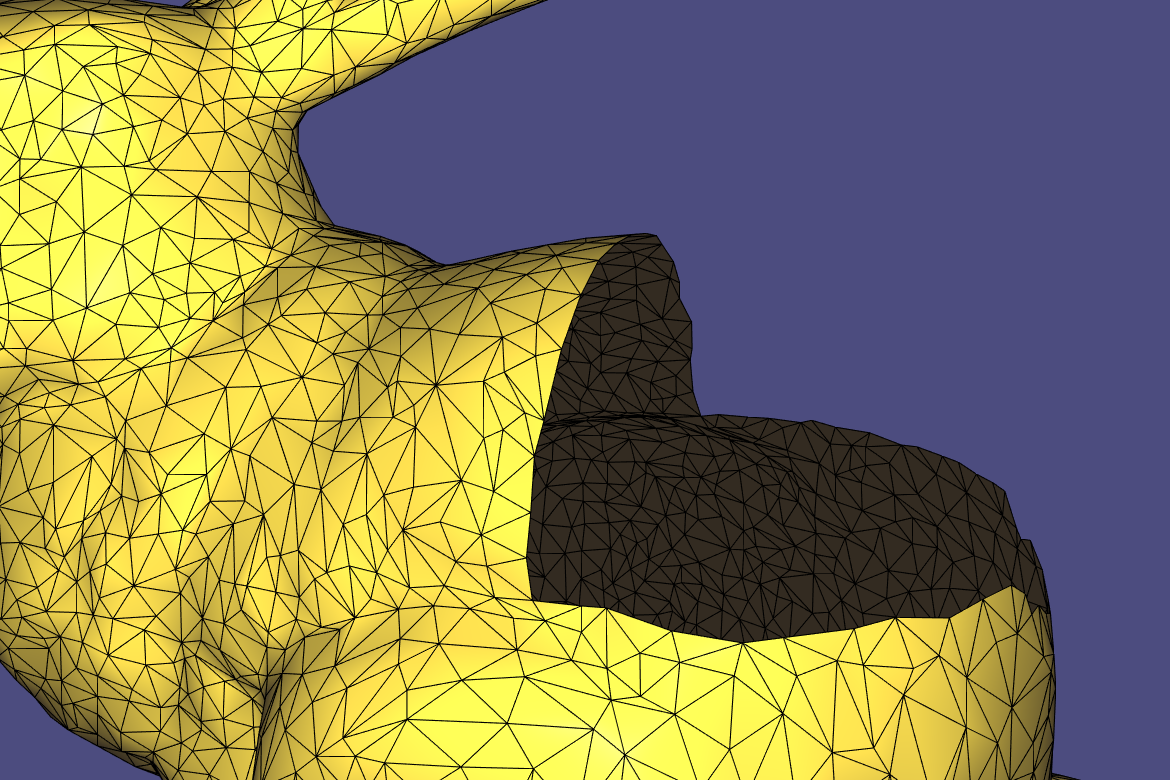Most of the techniques described in this article are based the description of Surface Fairing in section 4.3 of [1]. In the below image, it is shown how our described algorithm can be used to smoothly and naturally fill holes in a broken mesh.

Our Approach

First, we shall describe our general approach to solving the problem. Let us say we have some geometry with a hole, and from the side, it looks like this

As can be observed, we describe the height at every point with a function $f$, so that $f(1)$ is the height of the first vertex, and so on. At $x=1$, $x=2$, $x=7$ and $x=8$ there are vertices, but in between, there is a hole at $x=3$, $x=4$, $x=5$, $x=6$. We wish to add a patch of four vertices at these four points that fills the hole, and we also want to ensure the height of these vertices follows the general curvature around the hole. We will find these four heights by formulating a system of equations, and then solving it, so that the obtained solution is the values of $f(3)$, $f(4)$, $f(5)$ and $f(6)$.

What kind of solution would be a good and desirable solution? We claim a solution like the below is a good solution

While the below solution is a bad solution

In the bad solution, the patch that fills the hole, is simply a linear interpolation from $x=2$ to $x=7$. The issue with such a solution is that it poorly preserves the slopes(that is, the derivatives) of the surroundings of the patch. The derivative at some point $x$ can be approximated as \[ f_x(x) = \frac{f(x + h) - f(x)}{h} = f(x + 1) - f(x) \] where we have let the step size be $h = 1$, and where we are using the notation $f_x(x) = \frac{\partial f}{\partial x}$ to denote the first derivative with respect to $x$, and then the second derivative is denoted $f_{xx}(x)$. Observe that $f_x(1) = 5 - 2 = 3$. In the good solution, we have that $f_x(2) = 2.1$, but in the bad solution we have $f_x(2) = 0.2$. The derivative at $f_x(2)$ is much closer to the derivative at $f_x(1)$ in the good solution compared to the bad. The change in derivative is smaller for the good solution, and this results in the transition from $f(2)$ to $f(3)$ being a much more natural transition, since this transition is more consistent with the derivatives of the surrounding vertices. To summarize, we desire a small change in the value of the derivative, as we go from one vertex to its neighbour. The change of derivative is simply the second derivative, and we wish to minimize this quantity over the patch.

This point is very important and the key of the technique, so let us clarify it even more: the first derivative, $f_x(x)$, measures how the function $f(x)$ changes as we go from $x$ to $x+1$. Then the definition of the second derivative, $f_{xx}(x)$ , is obvious: it measures the change of $f_x(x)$ as we go from $x$ to $x+1$. In order to create a smooth patch that naturally follows the curvature around the hole, we will create a patch that minimizes the second derivative.

Minimizing the Second-Derivative with Variational Calculus

In this section, we will implement the approach described in the previous section. Our objective is to find some function $f(x)$, that describes a patch that has the requirements we described in the previous section. For the case of our example, we already know the values of this function for $x=1$, $x=2$, $x=7$ and $x=8$, but we need to solve and find the values for $x=3$, $x=4$, $x=5$ and $x=6$. The example function we have been dealing with up until this point has been a discrete function $f(x)$, that is only defined at the integers. We will now temporarily move from the discrete domain into the continuous domain, since this allows us to use the powerful tools of variational calculus. Henceforth, $f$ is not only defined for values such as $x=2$ and $x=6$, but also for values such as $x=1.2$ and $x=1.5$.

We wish to find a function $f(x)$, such that the second derivative is minimal at all points in the patch. Then it is natural to define the energy function \[ E(f) = \int_a^b (f_{xx})^2\ dx \] (This integral would not have been possible in the discrete domain!)The above integral can be seen as a sum. Put in a simplified way, it evaluates the value of $(f_{xx})^2$ at many, many points in the interval $[a, b]$, and then adds all these evaluations together into one large sum. If this integral is small, then the second derivatives in the interval $[a, b]$ will be small, and this means $f$ is a good patch by our requirements. Note that $a$ and $b$ are the boundary points of the patch, and the boundary is $x=2$ and $x=7$ for the example function.

In order to find the $f$ that minimizes $E(f)$, we utilize a common approach of variational calculus: First, we assume that $f$ is the minimizer of $E(f)$. Further, let $u(x)$ be any function that is defined in the interval $[a,b]$, and is once differentiable in this interval(this means that we can compute its first derivative in this interval), and that further satisfies $u(a) = u(b) = 0$ and $u_x(a) = u_x(b) = 0$. It will soon become clear why we are doing this.

Consider now the function $E(f(x) + u(x)\lambda)$. This is a function where we are adding a certain amount of $u(x)$ to $f(x)$ and then giving this sum to $E()$. How much of $u(x)$ that we add to $f(x)$ is controlled by the scalar $\lambda$. We assumed that $f(x)$ is the minimizer of $E(f)$, and this implies that $\lambda=0$ is the minimizer of $E(f(x) + u(x)\lambda)$. But this means that the derivative of $E(f(x) + u(x)\lambda)$ with respect to $\lambda$ must be $0$ when $\lambda = 0$(since the derivative is zero at the minimum point). That is \[ \frac{\partial E(f(x) + u(x)\lambda)}{\partial\lambda} \bigg\rvert_{\lambda = 0}= 0 \] We shall now expand and simplify the left-hand side. For convenience, we will onward write $u(x)$ as $u$ and $f(x)$ as $f$. First observe that \[ E(f + u\lambda) = \int_b^a ( (f + u\lambda)_{xx} )^2\ dx = \int_b^a (f_{xx} + u_{xx}\lambda)^2\ dx \] Next we compute the derivative with respect to $\lambda$. \[ \frac{\partial E(f + u\lambda)}{\partial\lambda} = \frac{\partial}{\partial\lambda}\left(\int_b^a (f_{xx} + u_{xx}\lambda)^2\ dx\right) = \int_a^b 2(f_{xx} + u_{xx}\lambda)u_{xx}\ dx \] (we have here performed differentiation under the integral, and this is completely acceptable by the Leibniz's rule). When $\lambda=0$, the right-hand side must equal zero, and thus it follows \[ \int_a^b f_{xx}u_{xx}\ dx = 0 \] Recall that $u(a) = u(b) = 0$ and $u_x(a) = u_x(b) = 0$. By using these facts and integration by parts, it is possible to simplify the above even further. Integration by parts yields \[ \int_a^b f_{xx}u_{xx} dx = [f_{xx}u_x]^b_a - \int_a^b f_{xxx} u_x\ dx = 0 \] However, $u_x(a) = u_x(b) = 0$, and thus it simplifies to \[ \int_a^b f_{xxx} u_x\ dx = 0 \] Integrate by parts again \[ \int_a^b f_{xxx} u_x dx = [f_{xxx}u]^b_a - \int_a^b f_{xxxx}u\ dx = 0 \] But $u(a) = u(b) = 0$, so we can simplify as \[ \int_a^b f_{xxxx}u\ dx = 0 \] Finally, here comes the coup de grace. Recall our definition of $u(x)$: it is any function that satisfies $u(a) = u(b) = 0$ and $u_x(a) = u_x(b) = 0$, and is once differentiable. How can we ensure that the above equality is satisfied, while still letting $u(x)$ be any function? The only possible way to satisfy such a strong condition, is by requiring that \[ f_{xxxx} = 0 \] That is, $f_{xxxx}$ must always be zero within our domain $[a,b]$. This implies that the minimizer of $E(f)$ is a function whose fourth derivative is always zero within the domain. We will use this fact to solve for the minimizer $f$ in the following section.

However, note that instead of solving for the $f$ whose fourth derivative with respect to $x$ is zero, we will find the $f$ whose bi-laplacian is zero, which is of course equivalent to the former. We are in this example dealing with only one dimension, and the laplacian in one dimension is simply $\Delta f = f_{xx}$. This means that our condition $f_{xxxx} = 0$ is equivalent to \[ \Delta\Delta f = \Delta^2 f = 0 \] where $\Delta^2$ is often called the bi-laplacian or the bi-harmonic operator, which is just the laplacian of the laplacian. The laplacian is more commonly used in notation than the fourth derivative, so this is why we are formulating our condition in terms of the laplacian.

Discretizing and Solving for the Minimizer

In the beginning, we showed a function with bar charts with a hole in it, and now we will show how to find the minimizer that fills this hole, and at the same time make sure that the second derivatives are minimal. The minimizer $f$ must satisfy the condition \[ \Delta\Delta f = \Delta^2 f = 0 \] However, this condition is in the continuous domain, and our bar chart is in the discrete domain, and so is a 3D mesh. In practical applications, discrete domains are very common, and so the bi-laplacian must be discretized. We will demonstrate how this can be done in the one-dimensional case. The bi-laplacian is the fourth derivative in one dimension. The first step is to discretize the first derivative, using central differences. \[ f_x(x) = \frac{f(x + 0.5h) - f(x - 0.5h)}{h} = f(x+0.5) - f(x-0.5) \] Where we used a step length of $h=1$, the smallest possible step length in our discrete problem. The second derivative, is the derivative of the first derivative \[ \Delta f(x) = f_{xx}(x) = f_x(x+0.5) - f_x(x-0.5) = f(x-1) - 2f(x) + f(x+1) \] Finally, the bi-laplacian is just the laplacian of the laplacian \[ \Delta^2 f(x) = f_{xxxx}(x) = f_{xx}(x-1) - 2f_{xx}(x) + f_{xx}(x+1) = f(x-2) - 4f(x-1) + 6f(x) - 4f(x+1) + f(x+2) \] Now we can finally solve for $f$ in our bar chart problem. First, observe that we desire to have $\Delta^2 f(3) = 0$. Using our discretization scheme, this can be simplified to \[ f(1) - 4f(2) + 6f(3) - 4f(4) + f(5) = 0 \] And same type of linear equation also holds for $f(4)$, $f(5)$, and $f(6)$. We summarize all these linear equations into a single matrix equation \[ \begin{bmatrix} 1 & 0 & 0 & 0 & 0 & 0 & 0 & 0 \\ 0 & 1 & 0 & 0 & 0 & 0 & 0 & 0 \\ 1 & -4 & 6 & -4 & 1 & 0 & 0 & 0 \\ 0 & 1 & -4 & 6 & -4 & 1 & 0 & 0 \\ 0 & 0 & 1 & -4 & 6 & -4 & 1 & 0 \\ 0 & 0 & 0 & 1 & -4 & 6 & -4 & 1 \\ 0 & 0 & 0 & 0 & 0 & 0 & 1 & 0 \\ 0 & 0 & 0 & 0 & 0 & 0 & 0 & 1 \\ \end{bmatrix} \begin{bmatrix} f(1) \\ f(2) \\ f(3) \\ f(4) \\ f(5) \\ f(6) \\ f(7) \\ f(8) \\ \end{bmatrix} = \begin{bmatrix} 2 \\ 5 \\ 0 \\ 0 \\ 0 \\ 0 \\ 6 \\ 3 \\ \end{bmatrix} \] Note that rows 1, 2, 7 and 8 simply specify the values at the boundaries of the bar chart. These are the boundary conditions of our problem, and must be specified in order to create a solvable equation. The remaining rows specify that the bi-laplacians of the unknown variables $f(3)$, $f(4)$, $f(5)$, $f(6)$ must equal zero. However, this matrix equation can be simplified. For row 3, we have \[ f(1) - 4f(2) + 6f(3) - 4f(4) + f(5) = 0 \] But since the values of $f(1)=2.0$ and $f(2)=5.0$ are known, we can move some constant values to the right-hand side, keeping only the variables on the left side: \[ 6f(3) - 4f(4) + f(5) = 18 \] We do the same for the other three linear equations, and remove rows 1,2, 7 and 8, since these rows are now redundant. Our simplified matrix equation is \[ \begin{bmatrix} 6 & -4 & 1 & 0 \\ -4 & 6 & -4 & 1 \\ 1 & -4 & 6 & -4 \\ 0 & 1 & -4 & 6 \\ \end{bmatrix} \begin{bmatrix} f(3) \\ f(4) \\ f(5) \\ f(6) \\ \end{bmatrix} = \begin{bmatrix} 18 \\ -5 \\ -6 \\ 21 \\ \end{bmatrix} \] If we solve, we obtain our solution below, which is also the good solution that we showed earlier.

Smooth 3D Hole-Filling Surface Patches

We have shown how to smoothly fill holes in the one-dimensional case. We will now briefly discuss how to smoothly fill holes in 3D meshes. Most of the reasoning from the one-dimensional case carries over to the 3D case, so this discussion will be more brief.

First, we locate the hole in the mesh. The below image illustrates this hole

and then compute the center position of the vertices in the hole boundary(this is the average of the vertex positions). The vertices in the boundary are connected with a newly created vertex at the center position, thus creating a surface patch that fills the hole. 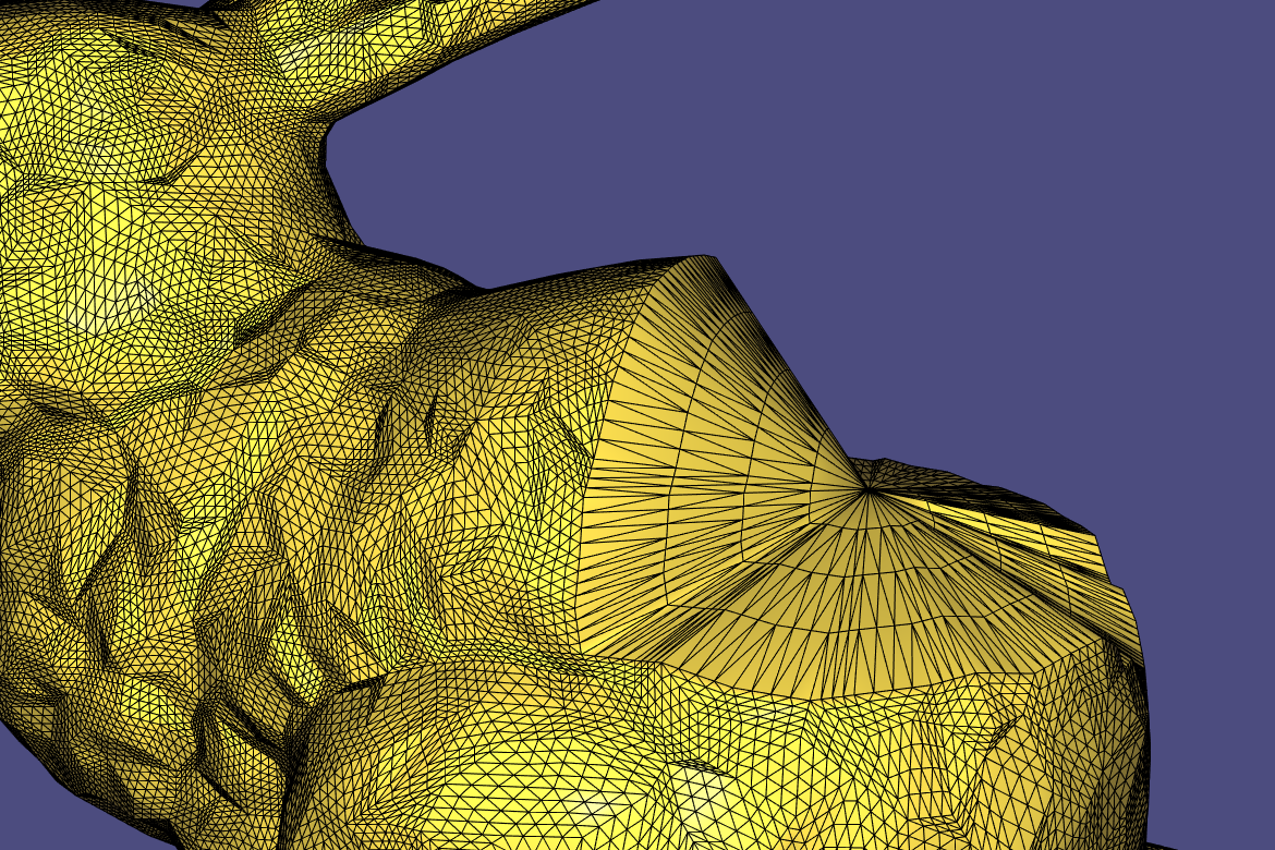The triangles in this patch are also upsampled(subdivided), so that we have more vertices to manipulate for when we will be making the patch more smooth. The result can be seen below

Note that we also upsampled the triangles of the original bunny mesh, since this makes it very easy to fuse together the vertices of the original patch and the original geometry. By "fuse", we mean that we ensure that the boundary of the original mesh, and the boundary of the patch share the same vertices.

Next, we create a smooth patch by solving the equation $\Delta^2 f = 0$ on the patch. We need to discretize the laplace operator to achieve this, and the discretization of the laplace operator on the surface of a mesh is called the Laplace-Beltrami operator. This is a topic that is too large to be covered in this article, and will probably be the subject of a future article. Instead, we mention that libigl provides code that creates the discretized Laplace-Beltrami operator, and then solves the equation $\Delta^2 f = 0$. 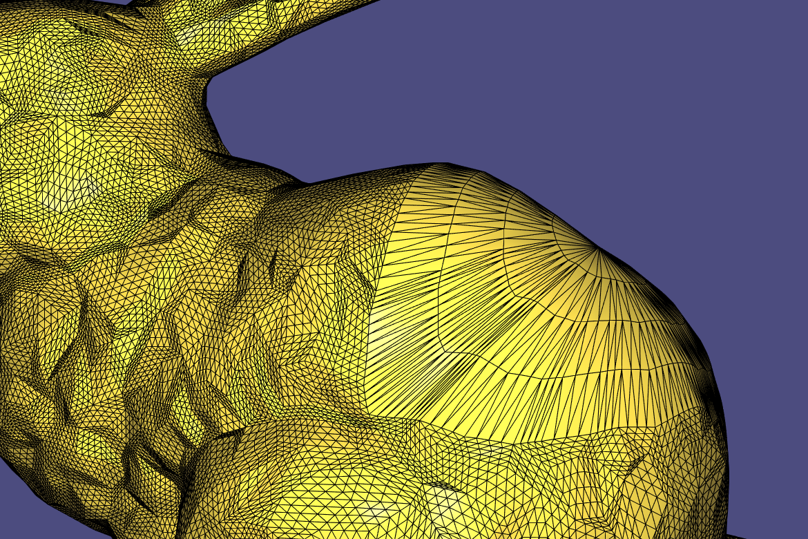This is what we used in our demo implementation of the technique. We solve for $f$, and the results can be seen below

Finally, we downsample the mesh, using a mesh decimation algorithm.

This concludes the article. In a github repository, we provide a commented implementation of the technique implemented with libigl and Eigen.

References

[1] Mario Botsch, Leif Kobbelt, Mark Pauly, Pierre Alliez, Bruno Lévy., "Polygon Mesh Processing".

The EVE Online Real Estate Crisis

Back in 2003 when I was helping CCP with their new economy in EVE Online, the biggest problem with their design was that the factories that were central to the player based economy were too cheap to buy and maintain. Since the game was released in the UK a day earlier than in the USA, by the time I was allowed to log into the retail version of the game all of the prime factories had been grabbed. This forced me to race to Minmatar space, where the ships were generally held in lower esteem by beta testers.

There I managed to buy the factories in a key star hub and set up shop. I produced the first Mammoths (a massive transport ship critical to trade) in the game, and also the first Minmatar battleships. I would have loved to expand my production but within days of the retail launch all factories had been bought up and idled by speculators who were charging $300 to $400 per factory, without any way of knowing if they really owned the factory or not.

One week after the launch of EVE I handed a report to Reynir Hardarson explaining, among other things, how this weakness in the economic design threatened their game and how to solve it. My solution was to greatly raise the rents on these factories so that only those that were actually actively running them would want to hold them. The idea was to create a “hot potato” effect where no rational person would want these factories unless they were doing a lot of output with them.

While it took several months to implement the fix, once it was in it worked perfectly by causing the speculators to abandon their stranglehold on the economy. In the meantime a handful of players who did have factories (myself included) got exceedingly rich. Thus the effect of this speculation was increased wealth stratification, reduced economic competition, increased consumer goods prices, and crazy real estate inflation.

Parallels in the “Real” Economy

When I began creating virtual economic systems and theories in 2005, I looked to the way our “real” economies were designed to see if I could find parallel systems. I wondered if excessively low property taxes would do the same thing in real life. The way this works is that if the tax or overhead on property is lower than the rate of increase of the value of that property, then this becomes an investment that generates profit. If the tax on property exceeds the value generated by appreciation, then this becomes a losing investment.

Because of this interaction, high property taxes reduce the value of property, again due to the “hot potato” effect. Low property taxes raise the value of property and trigger speculation. In a “high tax” environment, only those that really need the property will be motivated to hold it. Families would be a good example of a group that “needs” property, some place to live. In a low tax environment, speculation makes property values so high that people seeking homes have a hard time affording them.

I wanted to see how this translated to the real world so I looked around for examples. The most obvious such example was California's Proposition 13, which was passed in 1978 when I was only 12 years old. This not only lowered property taxes, but also increased property values as described above. Its effects were exactly what you would have predicted from the scenario generated in EVE Online.

There was one additional difference in the real world, however. EVE Online is not a closed system. By this I mean that when a tax or rent is paid in EVE, this does not cycle back into the economy, it just magically disappears. In the real world, when a property tax is paid it cycles back into the economy through expenditures on public infrastructure such as education and road maintenance. Thus when the property taxes were lowered the result was a widespread degradation in public infrastructure, an effect not observed in EVE. 

Real Estate Bubbles are Pyramid Schemes

When you speculate on real estate, you are gambling that the value of that real estate will continue to rise, at a rate greater than the overhead on that property. This does not occur unless the number of speculators increases over time, otherwise demand would stay flat and property values would not rise. A rapid influx of new residents in California would have also increased property values by increasing demand, but the population growth during this time was relatively flat in California.

A rapid increase in the pool of speculators allows each generation of speculators to unload their investments on the next generation and to generate a profit. Like all pyramid schemes, the system is unsustainable as it would need to approach infinity to continue. The faster the pyramid grows, the greater the profits for the early entrants, and the greater the losses for the last generation of participants (before the crash).

This pattern of real estate speculation in California is a basic part of life there. When a new “bubble” (this is what we like to call the pyramid in California) is forming you get a pattern like this: http://firsttuesdayjournal.com/the-rises-and-declines-of-real-estate-licensees/

Note the huge rise in real estate agents as the bubble heats up and approaches detonation. But this bubble was different. In 2006 I noted the proliferation of the Adjustable Rate Mortgage (ARM). Its use was increasing at a rate that was positively non-linear. The ARM is designed to let new players enter the pyramid that normally would not have the means to do so. This allows the pyramid to go on longer than it normally would, increasing the profits of early entrants. It also ensures that the last generation will be historically large.

Not only was the last generation of this pyramid unprecedented in size, but also in quality. These participants had little or no assets to give up when they got left holding overvalued property at the time the bubble burst. This means that the banks, who were seeking to profit off of the use of ARM's to foreclose on valuable California real estate, ended up with a massive amount of real estate that was not as valuable as they had hoped. It was “under water”. This further drove down property values, creating a negative feedback loop.

The result, which I predicted in 2006 in a conversation (and bet) with a friend who was a retired but powerful financial expert, was a system collapse that threatened to force our banking system to fail. This forces the government to step in to shore up the collapse. What is happening here is that the banks, the instigators of the ARM, did not realize that if the pyramid got too large they would end up being the last generation of the pyramid. Because the government feared what would happen if the banks collapsed, the government stepped in and volunteered to be the last generation of the pyramid.

You might find it interesting to note that I won that bet in 2008 by mutual agreement, and my friend fronted me the money I needed to return to school to study “real” economics. Now I consult to three international gaming companies with net revenues in excess of $1B each, as an applied virtual economist. Thank you CCP and EVE Online for teaching me so much.

Offentliggjort den 18. sep. 2014

(Submitted on 23 Feb 2018)

Abstract: The remarkable optical properties of the solar gravitational lens (SGL) include major brightness amplification (~1e11 at wavelength of 1 um) and extreme angular resolution (~1e-10 arcsec) in a narrow field of view. A mission to the SGL carrying a modest telescope and coronagraph opens up a possibility for direct megapixel imaging and high-resolution spectroscopy of a habitable Earth-like exoplanet at a distance of up to 100 light years. The entire image of such a planet is compressed by the SGL into a region with a diameter of ~1.3 km in the vicinity of the focal line. The telescope, acting as a single pixel detector while traversing this region, can build an image of the exoplanet with kilometer-scale resolution of its surface, enough to see its surface features and signs of habitability. We report here on the results of our initial study of a mission to the deep outer regions of our solar system, with the primary mission objective of conducting direct megapixel high-resolution imaging and spectroscopy of a potentially habitable exoplanet by exploiting the remarkable optical properties of the SGL. Our main goal was to investigate what it takes to operate spacecraft at such enormous distances with the needed precision. Specifically, we studied i) how a space mission to the focal region of the SGL may be used to obtain high-resolution direct imaging and spectroscopy of an exoplanet by detecting, tracking, and studying the Einstein ring around the Sun, and ii) how such information could be used to detect signs of life on another planet. Our results indicate that a mission to the SGL with an objective of direct imaging and spectroscopy of a distant exoplanet is challenging, but possible. We composed a list of recommendations on the mission architectures with risk and return tradeoffs and discuss an enabling technology development program.

In 2014, we began development on Heron, a real-time streaming and analytics platform, to reliably process billions of events generated at Twitter every day. Today, we are proud to donate Heron to the Apache Incubator where the community will continue to grow and thrive under the guidance of the Apache Software Foundation. We are excited to see usage of Heron grow beyond our use cases here at Twitter, and look forward to continued community growth and collaborative support.

Heron is the next generation distributed streaming engine that was built to be backwards compatible with Apache Storm, which we open sourced in 2011 and donated to Apache. It was built to improve our developer and operational experiences with Storm and introduced a wide array of architectural improvements and native support for Apache Aurora. Heron has become our primary streaming system, reliabily powering all of Twitter’s real-time analytics and running hundreds of development and production topologies deployed on thousands of nodes.

Twitter Heron galvanized the streaming community by introducing several new ideas in stream processing including:

• Backpressure to adjust the pace of execution of topologies based on slowest component.
• Notion of modularity similar to microkernels that allows multi language support and provide alternative implementations for module (for constantly changing big data landscape)
• Isolation at various levels for ease of debugging and troubleshooting
• Native containerization for supporting cgroups and dockers
• Process based as opposed to thread based for profiling and troubleshooting
• Support diverse workloads in a single deployment - latency sensitive vs throughput sensitive with simple configuration change at each topology.

In 2016, we were excited to open source Heron, which enabled the project to grow into the vibrant and active community it is today. Some of the significant contributions from collaboration with community include:

• New APIs. First, high level functional API called Streamlets have been introduced both for Java and Python. Second, low level API similar to Storm API have been added for Python. The key advantage is Python API based topologies run in native python interpreter and directly receive and process data. Furthermore, support for ECO (Extensible, Component, Orchestrator) API using YAML for topology stitching is provided.
• Incorporation of stateful and effective once processing with adaptors for Apache Hadoop, Apache BookKeeper, and local file system.
• In collaboration with Microsoft, Heron pioneered the work of Dhalion based on the operational experiences it went through. Dhalion allows Heron to self tune, self heal and self stabilize when the topologies experience unexpected behaviors due to system behavior and change in data rate and volume - without any manual intervention.
• Open source Heron includes optional storage called Apache BookKeeper that provides a seamless experience for distributing job jars and also serves as a stateful storage for exactly once processing.
• Support for several scheduler deployments such as Kubernetes, DC/OS, Nomad, SLURM and standalone thereby taking advantage of those scheduler features.

We’ve worked collaboratively with the open source community and have benefited from contributed features that are now running in production at Twitter. We shared our experiences in streaming by publishing several papers in premier conferences.

Thank you to the Real-Time Compute team at Twitter, and to the Heron Community, for your continued support as the project moves onto the next phase of its life-cycle. Please follow us on Twitter at @heronstreaming, subscribe to the mailing list, and help support Heron in its new home!

[1] Dhalion: Self-Regulating Stream Processing in Heron, Proceedings of the Very Large Database(VLDB), September 2017.

[2] Twitter Heron: Towards Extensible Streaming Engines, IEEE 33rd International Conference on Data Engineering (ICDE), May 2017.

[3] Optimizing Twitter Heron, Twitter Engineering Blog, March 2017.

[4] Open Sourcing Twitter Heron - Twitter Engineering Blog, May 2016.

[5] Streaming@Twitter, Bulletin of the Technical Committee on Data Engineering, IEEE Computer Society, December 2015.

[6] Twitter Heron: Streaming at Scale, Proceedings of ACM SIGMOD Conference, Melbourne, Australia, June 2015.

[7] Flying Faster with Heron, Twitter Engineering Blog, May 2015.

[8] Storm@Twitter, Proceedings of ACM SIGMOD Conference, Snowbird, Utah, June 2014.

• Major scientific breakthrough research has discovered new materials offering an alternative to battery power and proven to be between 1,000-10,000 times more powerful than the existing battery alternative - a supercapacitor
• The new technology is believed to have the potential for electric cars to travel to similar distances as petrol cars without the need to stop for lengthy re-charging breaks of between 6-8 hours, and instead re-charge fully in the time it takes to fill a regular car with petrol.
• The scientific findings made by Augmented Optics Ltd and its wholly owned subsidiary Supercapacitor Materials Ltd with the University of Surrey and University of Bristol have produced a safer, faster charging, more efficient and greener alternative to battery power and supercapacitor abilities as we currently know them.

Ground-breaking research from the University of Surrey and Augmented Optics Ltd., in collaboration with the University of Bristol, has developed potentially transformational technology which could revolutionise the capabilities of appliances that have previously relied on battery power to work.

This development by Augmented Optics Ltd., could translate into very high energy density super-capacitors making it possible to recharge your mobile phone, laptop or other mobile devices in just a few seconds.

The technology could have a seismic impact across a number of industries, including transport, aerospace, energy generation, and household applications such as mobile phones, flat screen electronic devices, and biosensors. It could also revolutionise electric cars, allowing the possibility for them to recharge as quickly as it takes for a regular non-electric car to refuel with petrol – a process that currently takes approximately 6-8 hours to recharge. Imagine, instead of an electric car being limited to a drive from London to Brighton, the new technology could allow the electric car to travel from London to Edinburgh without the need to recharge, but when it did recharge for this operation to take just a few minutes to perform.

Supercapacitor buses are already being used in China, but they have a very limited range whereas this technology could allow them to travel a lot further between recharges. Instead of recharging every 2-3 stops this technology could mean they only need to recharge every 20-30 stops and that will only take a few seconds.

Elon Musk, of Tesla and SpaceX, has previously stated his belief that supercapacitors are likely to be the technology for future electric air transportation. We believe that the present scientific advance could make that vision a reality. 

The technology was adapted from the principles used to make soft contact lenses, which Dr Donald Highgate (of Augmented Optics, and an alumnus of the University of Surrey) developed following his postgraduate studies at Surrey 40 years ago. Supercapacitors, an alternative power source to batteries, store energy using electrodes and electrolytes and both charge and deliver energy quickly, unlike conventional batteries which do so in a much slower, more sustained way. Supercapacitors have the ability to charge and discharge rapidly over very large numbers of cycles. However, because of their poor energy density per kilogramme (approximately just one twentieth of existing battery technology), they have, until now, been unable to compete with conventional battery energy storage in many applications.

Dr Brendan Howlin of the University of Surrey, explained: “There is a global search for new energy storage technology and this new ultra capacity supercapacitor has the potential to open the door to unimaginably exciting developments.”

The ground-breaking research programme was conducted by researchers at the University of Surrey’s Department of Chemistry where the project was initiated by Dr Donald Highgate of Augmented Optics Ltd. The research team was co-led by the Principal Investigators Dr Ian Hamerton and Dr Brendan Howlin. Dr Hamerton continues to collaborate on the project in his new post at the University of Bristol, where the electrochemical testing to trial the research findings was carried out by fellow University of Bristol academic - David Fermin, Professor of Electrochemistry in the School of Chemistry.

Dr Ian Hamerton, Reader in Polymers and Composite Materials from the Department of Aerospace Engineering, University of Bristol said: “While this research has potentially opened the route to very high density supercapacitors, these *polymers have many other possible uses in which tough, flexible conducting materials are desirable, including bioelectronics, sensors, wearable electronics, and advanced optics. We believe that this is an extremely exciting and potentially game changing development.”

*the materials are based on large organic molecules composed of many repeated sub-units and bonded together to form a 3-dimensional network.

Jim Heathcote, Chief Executive of both Augmented Optics Ltd and Supercapacitor Materials Ltd, said: “It is a privilege to work with the teams from the University of Surrey and the University of Bristol. The test results from the new polymers suggest that extremely high energy density supercapacitors could be constructed in the very new future. We are now actively seeking commercial partners in order to supply our polymers and offer assistance to build these ultra high energy density storage devices.”

For more details see www.Supercapacitormaterials.com

README.md

aws lambda invoke \
--invocation-type RequestResponse \
--function-name demo_lambda \
--region us-east-1 \
--log-type Tail \
--payload '{"key1":"value1", "key2":"value2", "key3":"value3"}' \
outputfile.txt

A few months ago I saw a great little blog post about state machines on the Shopify blog. The message was that state machines are great and developers should use them more – given my recent experiences with state machines at CrowdHired, I could certainly agree with that. But it got me thinking, how many times in my developer career have I actually used a state machine (either separate library or even hand-rolled abstraction)? The answer is zero times – which surprised the hell out of me since state machines really are very useful. So I decided to engage in a bit of introspection and figure out why we tend to manage our "state" and "status" fields in an ad-hoc fashion rather than doing what is clearly called for.

We Don't Need One Until We Do

The problem is that you almost never create an object fully formed with all the behaviour it is ever going to need, rather you build it up over time. The same is true for the "states" that a state machine candidate object can be in. So, early on you don't feel like your objects' state machine behaviour is complex enough to warrant a "full-blown" state machine (YAGNI and all that jazz), but later on – when it IS complex enough – you feel like you've invested too much time/effort to replace it with something that has equivalent functionality. It's a bit of a catch-22. It's overkill and by the time it's not, it's too late.

A State Machine Is A Fluffy Bunny (Not Particularly Threatening)

Those of us who went through computer science degrees remember state machines from our computing theory subjects and the memories are often not fond ones. There are complex diagrams and math notation, determinism and non-determinism, Moore and Mealy, as well as acronyms galore (DFA, NFA, GNFA etc.). We come to believe that state machines are more complex than they actually are and it is therefore nothing but pragmatism that makes us consider a "full-blown" state machine overkill.

But most state machines you're likely to need in your day-to-day development have nothing in common with their computing theory counterparts (except the … errr … theory). You have states which are strings, and events which are methods that cause transitions from one state to another – that's pretty much it (at least for the state_machine gem in Ruby). The point is, even if you have two states, a state machine is not overkill, it might be easier that rolling an ad-hoc solution, as long as you have a good library to lean on.

Even A Good Tool Is Not A Good Tool

I would hazard a guess that there are decent state machine libraries for most languages that you can use (the aforementioned state_machine for Ruby is just one example). But even a fluffy bunny has a learning curve (I am stretching the metaphor well past breaking point here). That wouldn't be such an issue if you were solving a problem, but all you're likely doing is replacing an existing solution. Since we tend to turn to a state machine library after the fact (our ad-hoc solution is working right now). Just like with everything that has "potential future benefits" the immediate value is very hard to justify even to yourself (unless you've had experience with it before). The slight learning curve only tips the scale further towards the "we can live without it" side. It doesn't matter how good a tool is if you never give it a chance.

It is really difficult to appreciate (until you've gone through it) – how much better life can be if you do give a good state machine library a chance. When we finally "bit the bullet" at CrowdHired and rejigged some of our core objects to use the state_machine gem, the difference was immediately apparent.

• Firstly the learning curve was minor, I did spend a few hours of going through the source and documentation, but after that I had a good idea what could and couldn't be done (I might do an in-depth look at the state_machine gem at some point). 
• The integration itself was almost painless, but moving all the code around to be inline with the new state machine was a big pain. In hindsight had we done this when our objects only had a couple of states it would have been a breeze. 
• We're now able to easily introduce more states to give our users extra information as well as allow us to track things to a finer grain. Before it was YAGNI cause it was a pain, now we find that we "ai gonna need" after all, cause it's so easy.
• Our return values from state transitions are now 100% consistent (true/false). Before we were returning objects, arrays of objects, nil, true/false depending on who was writing it and when. 
• We're now able to keep an audit trail of our state transitions simply by dropping in state_machine-audit_trail (see that Shopify post), before it was too hard to hook it in everywhere so we had nothing.
• We removed a bunch of code and improved our codebase – always worthy goals as far as I am concerned.

My gut-feel is that most people who read that Shopify post agreed with it in spirit, but did nothing about it (that's kinda how it was with me). We seem to shy away from state machines due to misunderstanding of their complexity and/or an inability to quantify the benefits. But, there is less complexity than you would think and more benefits than you would expect as long you don't try to retrofit a state machine after the fact. So next time you have an object that even hints at having a "status" field, just chuck a state machine in there, you'll be glad you did. I guarantee it or your money back :).

Image by tfangel

Jackson gave eloquent expression to a widespread sentiment in American culture: a fervent faith in the Bill of Rights—the Constitution’s first ten amendments—as our country’s most meaningful and effective limits on government power. Within these ten amendments, the thinking goes, can be found all of the essential safeguards against the tyranny of popular majorities. Jackson’s contemporary on the Court, Justice Hugo Black, referred to the Bill of Rights as “the heart of the Constitution.” President Truman venerated the first ten amendments as the Constitution’s “most important part,” guaranteeing “the right of the individual to go where he pleases, to do what he pleases, to say what he pleases.” It was these rights, Truman explained, that most clearly distinguished the United States from totalitarian states, where “the individual” has no choice but “to do what they tell him.”

Given the timeless quality of the rhetoric, one might assume that Americans have been venerating the Bill of Rights in an unbroken line since 1791. In a fascinating new book, The Heart of the Constitution: How the Bill of Rights Became the Bill of Rights, legal scholar Gerard Magliocca demonstrates the opposite. The modern idea of the Bill of Rights as the Constitution’s most important section, it turns out, is a surprisingly recent invention. For most of the nation’s history, in fact, the phrase “Bill of Rights” was not necessarily understood to signify the first ten amendments. Magliocca argues that both the precise definition and the larger meaning of the Bill of Rights have undergone reinvention throughout American history, invoked rhetorically to support competing positions in each new generation’s political controversies. And he worries that this process of reinvention may have stalled, with Americans now fetishizing the Bill of Rights, having lost sight of their own ability to remake the legal and political world.

Eighteenth-century Americans generally understood a bill (or declaration) of rights to constitute the prefatory sections of a constitution. In addition to their enumeration of specific protections, these bills also typically laid out broad, abstract principles. The paradigmatic example was the Virginia Declaration of Rights of 1776, which began by asserting that “all men are by nature equally free and independent” and endorsing the people’s “right to reform, alter, or abolish” governments deemed “inadequate” to the common good. Only then did the Virginia Declaration set about listing more specific guarantees, such as the right to a “speedy trial” and the protection against “cruel and unusual punishments.”

When the Anti-Federalists complained that the Constitution of 1789 lacked a bill of rights, then, they meant that it lacked a prefatory text along the lines of the Virginia Declaration of Rights. When the First Congress responded to these complaints by appending a list of amendments to the end of the Constitution, their handiwork was not immediately or widely regarded as a bill of rights. As Magliocca writes, the first ten amendments simply “did not match the eighteenth-century expectations” of what a bill of rights looked like. Madison himself referred to the proposed additions simply as “the plan of amendments.” According to Magliocca, only Jefferson denominated the first ten amendments as “the bill of rights” at the time, and even then, only in private correspondence.

Apart from a few fleeting references, the idea that the first ten amendments constituted the Bill of Rights lay dormant for most of the 19th century—as did the idea that the specific protections guaranteed within those amendments required robust judicial enforcement. After the Civil War, Congressman John Bingham promoted the idea that the first ten amendments constituted the Bill of Rights—and that the Fourteenth Amendment, which he helped to draft, expanded those amendments’ reach. Originally understood as limitations only on the federal government, the Bill of Rights should now, in Bingham’s view, be understood to bind the state governments as well. But the Supreme Court was not yet convinced; only in the 20th century would the Court grapple seriously with the arguments for “incorporating” the Bill of Rights against the states.

In Magliocca’s account, the 1940s marked the pivotal moment when Americans elevated the Bill of Rights to its current status as an object of legal, political, and cultural veneration. In 1941, Congress declared the first “Bill of Rights Day,” commemorating the 150th anniversary of ratification. In 1943, the Supreme Court issued its ruling in West Virginia v. Barnette, the Pledge of Allegiance case, and by the late 1940s, the Court routinely referred to the first ten amendments as “the Bill of Rights,” even as the justices continued to debate how to interpret and enforce those amendments.

Franklin Roosevelt was the first president to invoke the Bill of Rights repeatedly in his public speeches. Paradoxically, he celebrated the first ten amendments, which limit government power, in order to justify his unprecedented expansion of the federal government’s role. Roosevelt encouraged Americans worried about the New Deal to read “the Bill of Rights of the Constitution, which I have solemnly sworn to maintain,” and “ask yourself whether you personally have suffered the impairment of a single jot of these great assurances.” With the Bill of Rights in place, in other words, Americans had nothing to fear from expansive economic legislation or new federal agencies.

Although Roosevelt celebrated the Constitution’s limits on government, he also famously argued that modern life required a “Second Bill of Rights”: a set of positive entitlements to economic security and material well-being, including “the right to a useful and remunerative job,” “the right to adequate medical care,” and “the right to a good education.” This bill of rights, of course, never gained the same foothold in American political culture, and it gained no foothold at all in American law. To borrow Justice Jackson’s definition of a bill of rights, the subjects of employment, health care, and education were never “withdrawn … from the vicissitudes of political controversy”; to the contrary, they remain perennially debated and highly dependent on the outcome of elections.

In recent years, perhaps the most prominent critic of the cult of the Bill of Rights was Justice Antonin Scalia, who questioned whether Americans really understood how the Constitution worked to guarantee their liberties. “Most people think it’s the Bill of Rights” that protects their freedom, Scalia said, but “every tinhorn dictator has a Bill of Rights.” (Scalia frequently gave some version of this remark in his public appearances.) What really protects Americans from tyranny, Scalia believed, is the constitutional structure, the way that the Constitution distributes power across the branches and between the states and the federal government. “The Soviet Union had a wonderful Bill of Rights,” Scalia explained, but “it was worthless,” because with power totally centralized in the party, there was no way for the people to enforce their rights.

Magliocca offers a different criticism of Americans’ attachment to the Bill of Rights. If we are going to use that term to refer to the most important parts of our constitutional and legal tradition, Magliocca argues, then we have settled on far too limited a definition. “The Constitution does not state that the first ten amendments are the Bill of Rights,” Magliocca writes, nor, he argues, is there any good reason, historically or legally, to construe the term so narrowly. So yes, let’s celebrate the right to free speech and the protection against unreasonable search and seizure, but why not also celebrate “the abolition of slavery, the Fourteenth Amendment, [and] the Civil Rights Act of 1964”?

While reading Magliocca’s lively and thought-provoking book, I was reminded of something that the constitutional historian Jack Rakove once observed about the difference between the founding generation and our own. It is “curious,” Rakove said, that “in the 1780s Americans expressed confidence in their ability to devise new institutions of government as a supreme act of political wisdom, but today we are unable to imagine how we could ever improve upon what the framers did.” Drafting the Constitution, and its first set of amendments, “required a terrific amount of creative political thinking,” in Rakove’s words. “The framers were rethinking the nature of representative government, they were rethinking the nature of executive power, they were coming up with new rules for judges.” Perhaps we should fetishize the specific products of that creativity a bit less, and instead focus our admiration on the larger lesson that the Founders have to teach: that it is always possible to reimagine what politics and government might be.

Late July. New York City. A bedroom on the top floor of a four-story building in which I installed an air conditioner with several thousand too few BTUs. I barely know what a BTU is. The temperature that day reached into the upper 90s Fahrenheit, with humidity just short of actual water. The tiny weak air conditioner struggled to cool the room down while a few feet away I struggled to fall asleep. And yet I was unable to sleep without some sort of covering. In this case it was the barest edge of my lightest sheet, touching the smallest possible part of my torso.

Why this compulsion to be covered, however minimally, in order to sleep?

Blankets are common, but not universal, to humans during sleep, at least in the modern day. But historically, the effort involved in weaving large sheets put blankets at much too high a price point for most to afford. From the linen bedsheets of Egypt around 3500 B.C. to wool sheets during the Roman empire straight through to cotton in medieval Europe, bed coverings were for the wealthy.

By the Early Modern period in Europe, which followed the Middle Ages, production had increased enough so that more middle-class people could afford bedding, though not easily. “The bed, throughout Western Europe at this time, was the most expensive item in the house,” says Roger Ekirch, a historian at Virginia Tech who has written extensively about sleep. “It was the first major item that a newly married couple, if they had the wherewithal, would invest in.” The bed and bedding could make up about a third of the total value of an entire household’s possessions, which explains why bedsheets frequently showed up in wills.

In place of blankets and sheets, other sources of heat were common at night, usually from multiple people sharing a bed, or often livestock.

Today, there’s minimal anthropological work about bedding around the world. The best is a 2002 paper by Carol Worthman and Melissa Melby of Emory University, who compiled a study of sleeping arrangements in different parts of the world. “Recognition of the paucity of anthropological work on sleep is galvanizing: a significant domain of human behavior that claims a third of daily life remains largely overlooked by a discipline dedicated to the holistic study of the human condition,” they wrote. This passes for outrage in an academic paper.

The paper looked into some foraging and non-foraging peoples who live in hot climates near the equator, and found that only the nomadic foragers regularly sleep without bed coverings. Everyone else uses some form of covering, whether that’s plant matter or woven fabric, even in central Africa and Papua New Guinea, both tropical climates. Much more common than sheets or blankets are some form of padding; basically nobody sleeps simply on the ground as a matter of course.

As one more example of the goodness of blankets, there has also been a decent amount of research about the calming effect of weighted blankets, which can weigh up to 30 pounds. Studies indicate that they can curb anxiety and even be used in the treatment of autism.

“The requirement for blankets takes on two components to it,” says Dr. Alice Hoagland, the director of the insomnia clinic at the Unity Sleep Disorder Center in Rochester, New York. “There’s a behavioral component and a physiological component.” The latter is a little more clear-cut, so let’s dive into that first.

About 60 to 90 minutes before a usual bedtime, the body starts losing core temperature. There’s a physiological explanation for that: when the body is heated, we feel more alert. And conversely, when the body cools down, we tend to feel sleepier. Cooler internal body temperatures are correlated with a rise in melatonin, a hormone that induces sleepiness. A bunch of doctors tested this out by making people wear skinsuits—they kind of look like cycling outfits—that dropped their body temperature just a touch, one or two degrees Fahrenheit, to see if they’d sleep better. They did.

Your body’s ability to regulate its own heat gets way more complicated than that at night, though. Say you sleep for eight hours each night. In the first four hours, plus the hour or so before you fall asleep, your body temperature will drop a bit, from around 98 degrees Fahrenheit to around 96 or 97. But the second four hours are marked by periods of rapid eye movement (REM) sleep, a phenomenon in which most of our dreams take place, along with a host of physical changes.

One of those physical changes is an inability to thermoregulate. “You almost revert to a more, and this is my word, reptilian form of thermoregulation,” says Hoagland. She says “reptilian” because reptiles are unable to regulate their own body temperature the way we mammals can; instead of sweating and shivering, reptiles have to adjust their temperature through external means, like moving into the sun or into cooler shadows. And for those brief periods of REM sleep, we all turn into lizards.

Even in perpetually hot climates, nighttime temperatures drop, and the night is coldest, coincidentally, right at the time when our bodies are freaking out and unable to adjust to it. (The night is coldest right after dawn, in direct contradiction to aphorism.) So, like lizards, we have to have some way to externally regulate our body temperatures. You may think it’s unnecessary to use a blanket at 10 p.m., when it’s still hot, but by 4 a.m., when it’s colder and you’re unable to shiver? You might need it. So we may know from past experience that we’ll thank ourselves later for having a blanket, and thus force ourselves to use one (or at least have one nearby) when going to bed.

There’s more to it than that, though. Another strange thing that happens in the REM periods of sleep is that our bodies drastically lower their levels of serotonin, the neurotransmitter most associated with feelings of calm, happiness, and well-being. You know what’s associated with higher levels of serotonin? Blankets. Various studies have indicated that sleeping with a weighted blanket can trigger an uptick in the brain’s production of serotonin. So yet again, the blanket might be filling a need that our REM-addled brains create.

The other element that might explain our need for blankets is what Hoagland refers to as “pure conditioning.” “Chances are you were raised to always have a blanket on you when you went to sleep,” she says. “So that’s a version of a transitional object, in sort of Pavlovian way.” Basically, our parents always gave us blankets to sleep with—babies are a bit worse than adults at thermoregulation, meaning they get cold easily, meaning well-meaning adults put blankets on them—and so getting under a sheet or blanket is associated with the process of falling asleep. Instead of Pavlov’s dogs drooling at the sound of a bell, we get sleepy when covered with a sheet.

If you Google around for this question, you’ll end up with a bunch of theories about blankets simulating the warm, enclosed feeling we had in the womb. There could be some element of theoretical protection or security imbued by the blanket, which might be another bit of conditioning, but Hoagland thinks the womb comparison is pretty unlikely. “I’m very suspicious of anyone who implies that this goes back to the feeling of being in the womb,” she says. “I think that’s very far-fetched.”

Another possible reason is that blankets are soft and feel good. I could not find any studies that examine the question of whether people like blankets because they’re soft and feel good, so this may remain a great unanswered question.

Protocol aware recovery for consensus based storage Alagappan et al., FAST’18

Following on from their excellent previous work on ‘All file systems are not created equal’ (well worth a read if you haven’t encountered it yet), in this paper the authors look at how well some of our most reliable protocols — those used in replicated state machines (RSM) — handle storage faults and corruptions. The report is not good:

Our analyses show that most approaches employed by currently deployed systems do not use any protocol-level knowledge to perform recovery, leading to disastrous outcomes such as data loss and unavailability.

Aren’t these protocols (such as Raft and Paxos) explicitly designed to ensure agreement and tolerate failed nodes? The gold standard that you reach for when dealing with the most critical data that needs strong durability and consistency guarantees? Yes they are, but you always have to pay attention to the failure model the system is designed for. Storage faults and data corruptions weren’t part of that failure model. Somebody forgot to tell that to the real world.

Having demonstrated the problem, the authors go on to design a new protocol-aware recovery approach.

To correctly recover corrupted data from redundant copies in a distributed system, we propose that a recovery approach should be protocol aware. A protocol-aware recovery (PAR) approach is carefully designed based on how the distributed system performs updates to replicated data, elects the leader etc..

Failure to be protocol-aware might lead, for example, to a node attempting to fix its data from a stale node, potentially leading to data loss. The solution is CTRL, corruption-tolerant replication. It comprises a local storage layer that can reliable detect faults, and a distributed protocol to recover from them using redundant copies. The authors won a best paper award at FAST’18 for their work.

What could possibly go wrong?

Inside a storage device, faults manifest as either block errors or corruptions. Block errors arise when the device internally detects a problem with a block and throws and error upon access. Corruption can occur due to lost and/or misdirected writes and may not be detected by the device. Some file systems (e.g. btrfs) can detect corruption and return an error to applications. (See also ccfs ). Others, such as ext4, simply silently return corrupted data if the underlying block is corrupted.

In either case, storage systems build atop local file systems should handle corrupted data and storage errors to preserve end-to-end data integrity.

Keeping redundant copies on each node is wasteful in the context of distributed systems where the data is inherently replicated.

Within a replicated state machine system, there are three critical persistent data structures: the log, the snapshots, and the metainfo. The log maintains the history of commands, snapshots are used to allow garbage collection of the log and prevent it from growing indefinitely, and the metainfo contains critical metadata such as the log start index. Any of these could be corrupted due to storage faults. None of the current approaches analysed by the authors could correctly recover from such faults.

The authors conducted both a theoretical and practical (fault-injection) analysis of real world systems including ZooKeeper, LogCabin, etcd, and a Paxos-based system, resulting in a taxonomy of current approaches.

The first group of responses are protocol oblivious, of which the most trivial is no have no detection strategy at all and just trust the underlying file system. Slightly better is to use checksums to detect corruptions and crash the node on detecting an error. (LogCabin, ZooKeeper, etcd all crash sometimes when their logs are faulty, ZooKeeper also crashes on corrupt snapshots). Crashing harms availability, so another strategy is to truncate the log at the point of detection of faulty data. Unfortunately this can also lead to silent data loss if the recovering node form a majority with other nodes that are lagging (demonstrated in ZooKeeper and LogCabin). A more severe form of truncate is to delete and rebuild all data. This can also lead to data loss in a similar way.

Surprisingly, administrators often use this approach hoping that the faulty node will be “simply fixed” by fetching the data from other nodes.

Some protocol aware strategies include mark non-voting as used by a Paxos-based system at Google (a faulty node deletes all data on fault detection, and marks itself as a non-voting member). This can lead to safety violations when a corrupted node deletes promises given to leaders. Reconfiguring involves removing the faulty node and adding a new one but again can harm availability if a majority are alive but one node’s data is corrupted. BFT should theoretically tolerate storage faults, but is expensive.

In short, when we consider the simple set of sample scenarios shows below, it turns out that none of the existing approaches exhibit correct behaviour in all of them.

Only CTRL is able to ensure safety and high availability under all six of these scenarios:

Corruption-tolerant replication

CTRL extends the standard RSM fault model for crash tolerant systems with a storage fault model including faults both in user data and in file-system metadata blocks.

CTRL guarantees that if there exists at least one correct copy of a committed data item, it will be recovered or the system will wait for that item to be fixed; committed data will never be lost.

It’s the job of the local storage layer (CLStore) to reliably detect faulty data on a node. CLStore also needs to be able to distinguish between crashes and corruptions as otherwise safety may be violated.

For logs, CLStore uses a modified log format which includes persistence records written in a different part of the media to the main entries. On a checksum mismatch, if a persistence record is not present, then we can conclude that the system crashed during an update. One special case is when the corrupted entry is the very last one in the log. In this case CLStore cannot disambiguate, and marks the record as corrupted leaving it to distributed recovery to fix or discard the entry based on global commitment.

For snapshots, CLStore splits them into chunks so that a faulty snapshot can be recovered at the granularity of individual chunks.

For metainfo (which is special in that it cannot be recovered from other nodes), CLStore simply maintains two local copies. Since metainfo is small and updated infrequently this does not incur significant overhead.

To ensure that a faulty item, once detected, can be reliably identified (what if the identifier in an entry is corrupt?) CLStore also redundantly stores the identifier of an item apart from the item itself. Faulty data items and their identifiers are passed to the distributed recovery layer for recovery using RSM-specific knowledge.

Since metainfo files are recovered locally, the distributed recovery layer is responsible for recovering log entries and snapshots.

Recovering log entries

If a leader has no faulty entries, then fixing a follower is straightforward – the leader can supply them to the follower. Things get more interesting when the leader itself discovers a fault. Now we could run a leader election with the constraint that a node cannot be elected leader if its log contains a faulty entry. However, in scenarios such as those shown in (b) below, this will lead to otherwise avoidable unavailability.

So we relax the constraint, and allow a node to be elected leader even if it has faulty entries. However, the leader must fix its faulty entries before accepting new commands.

The crucial part of the recovery to ensure safety is to fix the leader’s log using the redundant copies on the followers… However, in several scenarios, the leader cannot immediately recovery its faulty entries; for example, none of the reachable followers might have any knowledge of the entry to be recovered or the entry to be recovered might also be faulty on the followers.

Known uncommitted entries (determined for example by checking that a majority of followers do not have the entry) can be safely discarded. A known committed entry (because one of the followers has a commit record) can be recovered from the follower with the record. When commitment can’t be quickly determined (nodes down or slow), then the leader must wait for a response.

In the unfortunate and unlikely case where all copies of an entry are faulty, the system will remain unavailable.

Recovering snapshots

Current systems including ZooKeeper and LogCabin do not handle faulty snapshots correctly: they either crash or load corrupted snapshots obliviously. CTRL aims to recover faulty snapshots from redundant copies.

In current systems, every node runs the snapshot process independently, taking snapshots at different log indices. This makes recovery complex. CTRL ensures that nodes take snapshots at the same index — identical snapshots enable chunk-based recovery. The leader announces a snapshot index, and once a majority agree on it, all nodes independently take a snapshot at that index. Once the leader learns that a majority (including itself) of nodes have committed a snapshot at an index i, it garbage collects its log up to i, and instructs the followers to do the same.

A leader recovers its faulty chunks (if any) from followers, and then fixes faulty snapshots on followers.

Recovery technique summary

The following table summarise the techniques used by CTRL for storage fault recovery.

Evaluation

I’m running out of space for today’s post, so will have to give the briefest of treatments to the evaluation. If you’re in any doubt about the need for a system like CTRL though, it’s well worth digging into.

The following table shows the results for targeted corruption testing using LogCabin and ZooKeeper — both in their original form, and retrofitted with CTRL.

Whereas recovery is theoretically possible in 2401 cases, the original systems are either unsafe or unavailable in 2355 of these. CTRL correctly recovers in all 2401 cases.

With block corruptions the original LogCabin and ZooKeeper are unsafe in about 30% of cases. With block errors, they are unavailable in about 50% of cases. CTRL correctly recovers in all cases:

With snapshot faults CTRL correctly recovers from all cases. Original ZooKeeper always crashes the node leading to unavailability and potential loss of safety. LogCabin is incorrect in about half of all cases.

In the face of file system metadata faults (e.g., corrupt inodes and directory blocks) CTRL will reliable crash the node, preserving safety.

When using SSDs, the throughput overhead of CTRL is 4% in the worst case.

The last word

Our work is only a first step in hardening distributed systems to storage faults: while we have successfully applied the PAR approach to RSM systems, other classes of systems (e.g. primary-backup, Dynamo-style quorums) still remain to be analyzed. We believe the PAR approach can be applied to such classes as well. We hope our work will lead to more work on building reliable distributed storage systems that are robust to storage faults.

"Column Tetris"

Actually, you can do something, but this needs deeper understanding. The keyword is alignment padding. Every data type has specific alignment requirements.

You can minimize space lost to padding between columns by ordering them favorably. The following (extreme) example would waste a lot of physical disk space:

CREATE TABLE t (
    e int2    -- 6 bytes of padding after int2
  , a int8
  , f int2    -- 6 bytes of padding after int2
  , b int8
  , g int2    -- 6 bytes of padding after int2
  , c int8
  , h int2    -- 6 bytes of padding after int2
  , d int8)

To save 24 bytes per row, use instead:

CREATE TABLE t (
    a int8
  , b int8
  , c int8
  , d int8
  , e int2
  , f int2
  , g int2
  , h int2)   -- 4 int2 occupy 8 byte (MAXALIGN), no padding at the end

As a rule of thumb, if you put 8-byte columns first, then 4-bytes, 2-bytes and 1-byte columns last you can't go wrong. text or boolean do not have alignment restrictions like that, some other types do. Some types can be compressed or "toasted" (stored out of line) or both.

Normally, you may save a couple of bytes per row at best playing "column tetris". None of this is necessary in most cases. But with billions of rows it can mean a couple of gigabytes easily.

You can test the actual column / row size with the function pg_column_size().
Be aware that some data types can use more space in RAM than on disk (compressed format). So you can get bigger results for constants (RAM format) than for table columns (disk format) when testing the same value (or row of values vs. table row) with pg_column_size().

SQL Fiddle.

Overhead per tuple (row)

4 bytes per row for the item pointer - not subject to above considerations.
And at least 24 bytes (23 + padding) for the tuple header. The manual on Database Page Layout:

There is a fixed-size header (occupying 23 bytes on most machines), followed by an optional null bitmap, an optional object ID field, and the user data.

For the padding between header and user data, you need to know MAXALIGN on your server - typically 8 bytes on a 64-bit OS (or 4 bytes on a 32-bit OS). If you are not sure, check out pg_controldata.

Run the following in your Postgres binary dir to get a definitive answer:

./pg_controldata /path/to/my/dbcluster

The manual:

The actual user data (columns of the row) begins at the offset indicated by t_hoff, which must always be a multiple of the MAXALIGN distance for the platform.

So you typically get the storage optimum by packing data in multiples of 8 bytes.

There is nothing to gain in the example you posted. It's already packed tightly. 2 bytes of padding after the last int2, 4 bytes at the end. You could consolidate the padding to 6 bytes at the end, which wouldn't change anything.

Overhead per data page

Data page size is typically 8 KB. Some overhead / bloat at this level, too: Remainders not big enough to fit another tuple, and more importantly dead rows or a percentage reserved with the FILLFACTOR setting.

There are a couple of other factors for size on disk to take into account:

Array types?

With array like you were evaluating, you would add 24 bytes of overhead for the array type. Plus, elements of an array occupy space as usual. Nothing to gain there.

Peter Thiel, never one to keep a low profile, made his most recent set of waves with reports that he is prepared to decamp from Silicon Valley to more benign haunts in Los Angeles along with several of his companies. His rationale, according to a piece in the Wall Street Journal, is that the Valley is now a politically intolerant culture, left-leaning in the extreme and to the exclusion of any contrarian viewpoints; any culture so unable to consider alternative viewpoints, the thinking continues, will stifle innovation. Thiel also is among the voices warning that the Valley is unprepared for a coming tsunami of regulations from Washington, which will undermine its ability to lead tech’s next wave.

Over the past decade, Thiel has proven to be a news magnet. He gets attention in the tech world much as Donald Trump gets attention in the political realm. Thiel speaks without a filter, often makes outrageous comments, and takes positions at odds with the elite—most notably his full-throated endorsement of Trump and a keynote at the Republican National Convention, when most of the technorati were card-carrying NeverTrumpers.

In this case, though, Thiel’s criticisms are themselves newsworthy. He may be an imperfect messenger, but his message had best be heard.

The size and scale of technology companies now surpasses that of most of the industrial, energy, and finance companies that dominated the American economy during the 20th century. The Valley’s close-knit groups of funders, founders, CEOs, and listed companies seem to think they can remain both insular and dominant without either government or social backlash. That was always far-fetched, and is now utterly absurd. It’s one thing for renegades to reinvent the operating system for society. But once those renegades become the rulers, the rest of society will—and should—demand a greater say in how these technologies and services shape our lives and consume our time, energy, and money.

Once upon a time—and in Valley-land, there is a once-upon-a-time—the tech ecosystem represented not just a small group of companies and funders, but also a relatively small slice of the nation’s economy. The early years of Apple, HP, and Intel may be looked at fondly and mythologized. But as recently as 1985, there was only one Valley company in the top 100 of the Fortune 500 list: Hewlett-Packard at No. 60. Xerox, based elsewhere but with a strong research presence in Palo Alto, was No. 38. IBM, based in New York, was then the largest tech company in the world. It clocked in at No. 6, and its rigid corporate culture and focus on selling to other corporations were seen as the antithesis to the Valley’s startup, countercultural vibe.

Even with the internet boom of the 1990s, the ethos of the Valley could rightly claim to be separate, new, and different, propagated by a band of misfits and upstarts, libertarian and utopian. Companies such as HP were more corporate and traditional, but the predominant meme was not just liberal and left, but dismissive of government, avid about a future where technology liberated all, and seemingly bemused by the vast wealth that these new products and services generated.

Today, however, some of those companies are more dominant than even the robber barons of old. At his apex, the oil billionaire J. Paul Getty was the richest man in the world, worth about $11 billion, adjusted for inflation. Today, there are 53 tech billionaires in California alone, and 78 in the United States; Jeff Bezos, Bill Gates (both of course in Seattle), and Mark Zuckerberg each have fortunes in excess of $50 billion. Peter Thiel has an estimated $2.5 billion.

That changes the equation, which Thiel implicitly realizes in his warning of coming regulation. It’s not just the personal fortunes, but the companies’ sheer scale and reach. Facebook connects nearly half the world’s adults, even if you adjust for inactive users. Google and Facebook together are a virtual duopoly for online ad sales; Amazon (again, not technically in the Valley but part of the equation) is racing ahead in e-commerce and cloud services; Salesforce, less mentioned because it is largely business-to-business, has established a preeminent market position with its sales and management software; Google’s YouTube is the entertainment hub for millennials and tweens. This list could go on for pages, and would only further illuminate just how dominant these firms have become. Add in the coming waves of artificial intelligence, with smart homes just the beginning, and the arc is for these companies to reach ever-deeper in our personal and professional lives.

That’s why there is and will be an even greater pushback against the idea that a small group of companies and executives can reap vast rewards, dictate the architecture of the online, cloud, AI, and robotic worlds and maintain an insular, parochial, and narrow worldview marked by groupthink.

For all of the libertarian gloss and utopian leanings, there are strong resemblances between today’s tech culture and the elites who dominated finance, business, and politics at the turn of the 20th century. Those elites had their moment as cultural icons, followed by intense pushback, vilification, and then regulation. J.P. Morgan was lauded for single-handedly bailing out the financial system from the Panic of 1907; barely five years later, he was hauled in front a congressional committee headed by Arsene Pujo of Louisiana, questioned about his leadership of a dark and secret “money trust” cabal, and cast as the villain of elite wealth who was defrauding the American people.

In his unartful way, then, Thiel is warning that the Valley’s tech elites are arrogantly unprepared for what’s coming. The government is eyeing them for the same reason robbers target banks: That’s where the money is. Tech will have an opportunity to shape the likely regulation, but only if it acts, rather than reacts, and offers real solutions that take the concerns of both government and citizens more seriously.

Where Peter Thiel lives is of at best marginal import to anyone but him. But his warning should be heeded now, while the Valley still has a chance to steer a new course and before the joystick is seized by others.

In Brief

Atacama Analogue

When we think of the potential for life on planetary bodies besides Earth, we automatically look for water. Whether it be growing at the bottom of Europa’s ocean or swimming in Titan’s methane lakes, we look for liquid because we understand the origins of life on Earth likely hinged on its abundant water. But a new study, led by scientists at Washington State University (WSU), suggests that life could exist with minimal water, even on planets as dry as Mars.

Published in the Proceedings of the National Academy of Sciences, the study examined the driest corner of the world’s driest desert — South America’s Atacama Desert. Here, decades pass with no rain, and it’s dry enough to be analogous to the surface of Mars.

Scientists have known that microbes exist in these extremely arid conditions, but they have been previously unsure of whether the microbes actually reside in this environment or are simply temporarily moved there by weather patterns. Within this study, the researchers concluded that this desert actually supports permanent microbial life.

The research team visited the Atacama in 2015 following an extremely rare rainfall, and detected a veritable boom of microbial life in the soil afterwards. When the team returned over the next two years, their samples showed the same microbial communities were still there, but had begun to dry out and go dormant, awaiting the next rain.

Martian Conditions

“It has always fascinated me to go to the places where people don’t think anything could possibly survive and discover that life has somehow found a way to make it work,” said Washington State planetary scientist Dirk Schulze-Makuch, in a press release. Schulze-Makuch led the study as part of his research into Earth’s most extreme organisms, which could tell us something about life through our universe.

“Jurassic Park references aside, our research tell us that if life can persist in Earth’s driest environment there is a good chance it could be hanging in there on Mars in a similar fashion,” he said.

This doesn’t mean that Mars is secretly teeming with life. However, it does point to the possibility. Because the Red Planet once held liquid water, Mars bacteria could have developed and then, as the planet dried out, evolved to adapt to a niche below the surface. Because Mars is so much colder, similar communities would likely have to live off the occasional melting of soil ice or snowfall on the surface.

The Washington state team will next be exploring extremely cold and salty locations on Earth to study more environments that could parallel those on Mars.

“There are only a few places left on Earth to go looking for new lifeforms that survive in the kind of environments you would find on Mars,” Schulze-Makuch said. “Our goal is to understand how they are able to do it so we will know what to look for on the Martian surface.”