README.md

# Debian based distros
sudo apt-get install ffmpeg zlib* libjpeg* python3-setuptools
# Mac
brew install ffmpeg zlib libjpeg python

sudo easy_install3 pip
# this should enable a pre-built Pillow wheel to be installed, otherwise you may need to install zlib and libjpeg development libraries so Pillow can compile from source.
pip3 install --user wheel

python3 setup.py install --user

pip3 install --user gif-for-cli

# Linux
if [ -d "$HOME/.local/bin" ] ; then
    PATH="$HOME/.local/bin:$PATH"
fi
# Mac, adjust for Python version
if [ -d "$HOME/Library/Python/3.6/bin/" ] ; then
    PATH="$HOME/Library/Python/3.6/bin/:$PATH"
fi

gif-for-cli path/to/some.gif
gif-for-cli http://example.com/foo.gif
gif-for-cli http://example.com/foo.mp4

python3 -m gif_for_cli path/to/some.gif

# get current top trending GIF
gif-for-cli

# get top GIF for "Happy Birthday"
gif-for-cli "Happy Birthday"

# get GIF with ID #11699608
# browse https://tenor.com/ for more!
gif-for-cli 11699608
gif-for-cli https://tenor.com/view/rob-delaney-peter-deadpool-deadpool2-untitled-deadpool-sequel-gif-11699608

gif-for-cli --display-mode=nocolor 11699608
gif-for-cli --display-mode=256 11699608
gif-for-cli --display-mode=256fgbg 11699608
gif-for-cli --display-mode=truecolor 11699608

gif-for-cli --rows 10 --cols 100 11699608

gif-for-cli --rows `tput lines` --cols `tput cols` 11699608

gif-for-cli -l 0 11699608

gif-for-cli --help

python3 -m unittest discover

coverage run --source gif_for_cli -m unittest discover
coverage report -m

git config core.hooksPath git-hooks

-bash: gif-for-cli: command not found

gif-for-cli 10988977
gif-for-cli 5863633
gif-for-cli 5437241

A program that implements the NIST 800-63-3b Banned Password Check using a bloom filter built from the Have I been pwned 2.0 SHA1 password hash list. The Have I Been Pwned 2.0 SHA1 password hash list contains more than 500 million hashes and is 30GB uncompressed (as of June 2018). The bloom filter of these SHA1 password hashes is only 860MB and will fit entirely into memory on a virtual machine or Docker container with 2GB of RAM.

SHA1 hashes are 20 bytes of raw binary data and thus typically hex encoded for a total of 40 characters. Blooming Password uses just the first 16 hex encoded characters of the hashes to build the bloom filter and to test the filter for membership. The program rejects complete hashes if they are sent.

False positive rates in the bloom filter are not impacted by the shortening of the SHA1 password hashes. The cardinality of the set is unchanged. The FP rate is .001 (1 in 1,000).

It's the simplest, smallest and fastest way to accomplish this sort of check. It can easily handle billions of banned password hashes with very modest resources. When a test for membership returns 404 then it's safe to use that password.

        $ cut -c 1-16 pwned-passwords-2.0.txt > 16.txt

        $ wc -l pwned-passwords-2.0.txt 
        501636842 pwned-passwords-2.0.txt

        $ sort -T /tmp/ -u 16.txt | wc -l
        501636842

        $ head 16.txt 
        7C4A8D09CA3762AF
        F7C3BC1D808E0473
        B1B3773A05C0ED01
        ...

• load /path/to/16.txt /path/to/output.filter

Send the first 16 characters of the hex encoded SHA1 hash to the Blooming Password program. Some examples using curl:

• curl -4 https://www.bloomingpassword.fun/hashes/sha1/0123456789ABCDEF
• curl -6 https://www.bloomingpassword.fun/hashes/sha1/F7C3BC1D808E0473

• 200 - The hash is probably in the bloom filter.
• 400 - The client sent a bad request.
• 404 - The hash is definitely not in the bloom filter.

In the 1960s, Dom Sylvester Houédard, a Benedictine monk who lived most of his adult life at Prinknash Abbey in Gloucestershire, England, would sneak off on weekends to London, where he participated in the emerging concrete poetry scene. This backstory is certainly alluring and unusual, and upon learning it at his current show at Lisson Gallery, one scours the works for signs of religious piousness.

Though they are littered with references to god and prayer (“prayersticks” (1969); “the jesus christ light and power company inc.” (1971); “RED God” (1967), to list a few), Houédard’s texts drip with humor more so than traditional religious devotion. (He called them “typestracts,” concrete poetry created using a typewriter, and “laminates,” collages of magazine words sandwiched between laminate paper.) And while clever, his works are also sincere. Houédard spent time in Asia while serving with the British military and was deeply influenced by Eastern philosophy. The geometric shapes, centered and minimal compositions, and simplistic color choices are balanced, beautiful, and even utopian. His color palette of mostly blues, reds, and blacks evokes Mondrian and the De Stilji artists who used abstraction to elevate their artwork towards the spiritual. “To be creative through the arts means that you are actually responding to your inner spaces,” notes Charles Verey, biographer and scholar of Houédard, in the accompanying catalogue, “so there’s a very close connection actually, between spirituality and the spirit of creativity.”

Houédard’s cut-and-pasted magazine collages recall Dada chance poems; his phrases are rooted in the counterculture movement of which he was a part. Friends with Allen Ginsberg and William Burroughs, “dsh,” as he signed his works, spent much of his time in London, at the home of Lisson gallerist Nicholas Logsdail and his partner Fiona McLean. According to Logsdail, and many others, Houédard referred to himself as a “monknik,” a title that reconciled his identity as a religious figure with his Beatnik interests and lifestyle.

Despite his phrases having been written long before iPhones, they remind me of text messages and experiences with autocorrect. I cannot count the number of times, while rushing down the street, I’ve sent a quick text to a friend to inform them of my delay only to look at it moments later and see the message looks nothing like what I wrote. “Bushmen impose their verbal clicks on zulus,” could easily be a line from one of such garbled messages. But unlike these messages, Houédard’s titles are deliberately chosen. This text, in a 1971 work, appears in all lowercase — as with most of his typestracts — justified slightly to the right, just above the center of a roughly letter-sized, off-white page. Above the text is a blue square filled with lines that appear to vibrate as they crisscross. This kind of movement is present throughout his images. In another 1971 work with a similar composition, “the jesus christ light and power company inc.,” the vibrating square is cut across with what looks like a lightning rod, made by gaps in the dashes. Houédard’s precise mark making creates a still image that moves and floats on the page. Language is never still.

Houédard’s laminated collages, visually very different than the typed works, also display slippage and movement. The glossy contact paper that holds them together makes them glisten in the gallery lighting, fitting considering Houédard was called these “cosmic dust laminate poems.” This is especially clear in “TULIP LABEL” (1967), which places his gridded geometric forms against a background of dust and various speckled materials, giving an otherworldly quality to the list of collaged words which hover over an atmospheric space: TULIP LABEL, BRONZE LABEL, OLIVE LABEL, GOLD LABEL, EMERALD LABEL, CRIMSON LABEL, WHITE LABEL, and DIAMOND LABEL. In her essay for the catalogue, Laura McLean-Ferris describes the fluid quality of these works: “Language slithers and puddles, bubbles slide down washed dishes, words and rain commingle with drips and jewelry.” Language is certainly a slippery form. Hard to pin down, easily muddled up, and easily miswritten, especially with the aid of our correcting machines.

The essays in the catalogue speculate as to why there has been a recent resurgence in interest in Houédard. They connect it to a rising awareness of the counterculture’s relationship to Eastern religion and spirituality. While that is perhaps what’s causing curators and researchers to bring his work more to light (with the publication of a scholarly monograph in 2012, in addition to a 2017 solo show at London gallery Richard Saltoun with an accompanying publication by Ridinghouse), it is its relevance to concerns of modern communication that give it staying power. Houédard wrote of concrete poetry: “concrete fractures linguistics, atomises words into incoherence, constricting language to jewel-like semantic areas where poet & reader meet in maximum communication with minimum words.” We are in an age of maximum communication with minimum words. But unlike poetry, our quick words tend to fail as we are bombarded by fake news, Twitter bots, and fast replies. Houédard, like other concrete poets, forces us to slow down how we read and see, his vibrating visuals and witty texts opening up the space between words and meaning.

Dom Sylvester Houédard continues at Lisson Gallery (136 10th Ave, Chelsea, Manhattan) through June 16. 

I've used Macs as my primary computing devices my entire life. And though I continue to use a Mac for my primary workstation for both work and personal projects, my use of computers has evolved in the past few years quite a bit. With more of my stuff moving into the cloud and fewer software applications being exclusively tied to macOS or Windows, it's given me more freedom to do some amount of work from a tablet (currently iPad Air 2), Mac (currently 2015 (work) or 2016 (personal) MacBook Pro), and even my old PC laptop (a Lenovo T420 that I used mostly for testing).

After lugging the T420 with me to an open source conference a couple weeks ago, I decided I'd finally go ahead and acquire a modern, Ultrabook-style Windows laptop, and looking around at options for an open source developer more comfortable in Linux than Windows 10, I narrowed it down to:

• Lenovo ThinkPad Carbon X1
• ASUS ZenBook
• Dell XPS 13

I settled on the Dell XPS 13 after reading through a bunch of reviews, looking at the features vs. size and battery life (I really value a compact laptop, especially coming from the behemoth T420!), and especially finding a really good price on a used 9360 model.

The model I purchased has the following specs:

• Intel Core i5-7200U - 2.50 GHz dual-core
• 8 GB LPDDR3-1866MHz RAM
• 120 GB SK Hynix SC311 SSD
• FHD (1080p) InfinityEdge display
• Intel HD Graphics 620
• 720p integrated webcam
• Windows 10 Professional

It's basically the base model, but I easily upgraded the SSD to a 500 GB model (see my experience upgrading the SSD here). I would've preferred 16 GB of RAM since I want to do some development and testing on the laptop... but that puts it in a price bracket I can't justify for a secondary computer mostly used for research and testing!

Hardware Build Quality

The fit and finish of the XPS lineup was one of the major reasons I chose it over the other models on my shortlist. I like a solid but light laptop, and the laptop against which I'll measure all others is still the 11" MacBook Air—if Apple would update it with a retina display and a larger 12" screen with a smaller bezel (so, basically, the 12" MacBook but with passable specs), I'd dump my MacBook Pro in a heartbeat! Note also that the XPS 13 is as wide as the 2016 MacBook Pro 13", but is very slightly thinner in the front (and slightly thicker in the back), and a little shorter front-to-back:

The Dell XPS 13 is a very nice piece of hardware—dare I say the best hardware of any PC laptop I've used or tried so far. The InfinityEdge display means the bezel is tiny, meaning the footprint is tiny. The aluminum front and back feel high quality and durable, like my MacBook Pro. There's a good balance and weight to it overall, and the rubber feet keep it solidly in place on any surface I've used it on so far.

There are three points about the hardware that were less-than-perfect, though:

The carbon fiber interior palmrest: When I opened the XPS the first time, I immediately noticed that my thumbprint remained after I opened the laptop. It's a little annoying—I don't have super-oily fingers, and have never had issues with other laptops (either hard plastic like the T420 or the cold aluminum of a MacBook Pro)—but I find myself wiping down the palmrests on the XPS 13 every hour or two, just because the finger prints make it look like I just ate a Whopper or Big Mac and wiped my greasy fingers on the surface!

The hinge mechanism: Speaking of opening the XPS—this is definitely a two-handed operation. And unlike the MacBook Air and Pro, there's no 'lip' in the frame with which you can easily slide a finger under the edge of the screen and pull up. So it's a little awkward in some situations where I'm used to one-handed operation (e.g. holding a drink, or positioning the laptop quickly while I'm holding something else). It's not a huge deal, but it is a mark against the laptop in my book.

The Keyboard: The keyboard hearkens back to the 2012-2015 'chicklet' style key action I was used to from the MacBook Pro line. It's slightly more refined than what I'm used to from a MacBook Air, but there is a lot of space between the keys, in the 'gutters'—enough so that I had to consciously move my pinky a tiny bit to get more accurate hits on the left Shift key. Apparently my fingers are optimized for the Shift key's edge to be a millimeter or so closer to the Z.

Trackpad

The trackpad is such an essential component of modern laptop usage (unless you're using it as a desktop replacement exclusively) that it warrants its own discussion. And, as someone who is used to the crème de la crème of laptop trackpads (Apple's glass Force Touch trackpad), a bad trackpad experience really puts me off the entire experience of using a laptop. My number one gripe with my old T420 was the trackpad, with it's finger-bludgeoning dotted/textured surface, and tiny tracking area (compared to most newer laptops).

The XPS 13 has a decent-sized trackpad, which is much wider than it is tall (following the aspect ratio of the display, it seems), and it has a very nice tracking surface. As close to Apple's glass surface as any I've used. It's not a Force Touch trackpad with haptic feedback, but rather a traditional trackpad with a physical clicking mechanism in the bottom left and right corners.

The software controls are pretty flexible, allowing 1-5 finger gestures (at least with Windows 10), and I don't really have much to complain about. The force required to physically click (I detest tap-to-click!) is a tad bit more than I'd prefer, but again, I've been pampered by Apple's Force Touch trackpads, which allow for different 'physical' click sensitivity settings.

Bottom line: This is the best trackpad I've used in a PC laptop, but it's still lacking a little in comparison to the best trackpad designs (IMO) from Apple.

Using the Apple Magic Trackpad 2 with Windows 10

Before wrapping up the trackpad discussion, I wanted to mention how I'm using my external Magic Trackpad 2—my favorite pointing device for any computer I've used—with the Dell XPS 13, because for many a Mac user not used to using Apple devices with Windows, they might not realize you can still use all the features of your fancy Apple hardware—just with a little more effort than would be required with most 'Made for Windows' accessories.

For those using Boot Camp on a Mac, and booting Windows 10 on a Mac itself, Apple's own (somewhat limited) Boot Camp control panel for Windows allows some controls over gestures, right click, sensitivity, etc.

But for those using PC hardware, the Boot Camp control panel won't help much. Instead, I've chosen to rely on a third party utility, the Magic Trackpad 2 Control Panel from Magic Utilities. It's a paid extension, but it provides control over every aspect of the Magic Trackpad 2.

Display

If I were buying the XPS 13 as my only laptop, I'd be a little more picky about the display. Having used high quality LG 4K external displays, and the Retina display on the 2015 and 2016 MacBook Pro, my standards for a display are pretty high; I do a decent amount of photography work, and when processing photos from my 24 Megapixel Nikon D750 and Sony a6000, I need as sharp and color-accurate a display as possible.

The XPS 13's FHD ('Full HD', or 1080p (1920x1080)) display is very good. Definitely a step down in color range and sharpness from the display in both my Retina MacBook Pros, but it's very good nonetheless. 1080p is a good tradeoff between resolution, battery life, and GPU performance, and the resolution is close enough to 'retina' quality that I'm satisfied for development work or day-to-day use.

Dell also offers a 4K display option, but according to various reports, it eats into battery life, has an even narrower color gamut, and in this form factor, is a little too much resolution to make a huge difference. It also adds a bit more to the cost, so it's probably not worth the tradeoffs just to get the extra pixels on a 13" display.

I/O Ports and Thunderbolt 3

One of the few major benefits of the newer MacBook Pros with only Thunderbolt 3 connectivity is I've finally reached my laptop-as-desktop nirvana state of only having one cable to plug into my laptop to provide:

• Power for charging
• 4K monitor connection (with 60 Hz refresh rate)
• USB 3.0 for keyboard, trackpad, SD card reader, and portable hard drives
• 1 Gbps Ethernet

In the past, I had setups where I had two or three cables to plug in whenever I put my laptop on my desk. Or I'd have a large and kludgy docking station. But no longer; now I have one cable sitting on my desk, and I plug it in to get all the connectivity I need. I am currently using the Elgato Thunderbolt 3 Dock, which cost $300, but can be hard to find in stock.

Can the Dell XPS 13's Thunderbolt 3 port do the same thing? You bet!

It's really awesome to be able to unplug my MacBook Pro, then plug in the XPS 13, and have the exact same setup with my external monitor, keyboard, and trackpad (and all the other peripherals).

One gripe with this experience, though, which has nothing to do with the hardware: the first time you plug in a dock to the Thunderbolt 3 port, Windows 10 spends about 5 minutes (literally!) identifying a bunch of new devices and adding them to the system, with a notification popping up for each thing. And unlike the Mac, where a couple seconds after you plug it in (even the first time), the new peripherals are usable, with Windows the new peripheral isn't usable (e.g. the display doesn't show an image, the trackpad doesn't track, the keyboard doesn't type) until Windows is finished setting up each device... one at a time. So the first time I plugged in the Dell, I thought the Thunderbolt 3 port might've been broken. Luckily it's just Windows' usability that's broken, but I knew that already ;-)

The XPS 13 also has a traditional barrel plug for AC charging, and comes with an old fashioned two-piece charging adapter. It has a charging light, but unlike the Magsafe connector I'm used to, it's just 'on' or 'off' (no multi-color charging status indication). There is a little button and 5 LEDs on the left side of the computer where you can quickly check battery charge status, though the LEDs seemed quite dim to me (you have to look head-on to see how many are lit).

Overall, the I/O situation on the XPS 13 is great for the size of the laptop, especially considering there's a Thunderbolt 3 connector in addition to an SD card reader, two USB 3.0 ports, an AC charging port, and headphone jack.

Battery Life and Thermal Management

Battery life, in my limited and non-scientific testing, has been excellent. Since this is a secondary laptop, I usually pull it out for a day's work, then plug it in to re-charge the battery, put it on my shelf for a week or two, then use it again another day. I've never run out of battery in a normal day's work so far, and just like the 2015 and 2016 MacBook Pro, the battery life is good enough that I don't really worry about bringing a charger anywhere unless I am planning on running tons of builds (e.g. Docker images or VM builds), or need to charge it up overnight.

In my normal day-to-day use (watching videos, streaming music, reading, programming), the battery will easily last all day, even with the screen at maximum brightness.

Unlike most PC laptops I've used, the thermal management is pretty good too; no area of the laptop heats up enough to burn my skin, and the XPS 13 never seems to turn into a small space heater (like my ThinkPad used to do quite often... even when idle!).

However, the XPS 13's fans do kick in quite often, even when just doing light tasks like browsing the web or typing. I was hoping it would be more like the MacBooks, which usually won't need to ramp the fans up to an audible level unless you're doing heavier work, like encoding a video or loading a news site web page without an ad blocker... but alas the fans often kick in and are audible during normal usage.

So, the XPS 13's battery life is excellent, but overall thermal management is just decent.

Built-in Webcam Nose-cam

It seems like every flagship laptop design has a major achilles heel. For the TouchBar MacBook Pro... it's the TouchBar. For the Dell XPS 13, it's the webcam. Don't take my word for it, though—every single review I found had a similar reaction to the webcam:

"And then there’s the placement of the webcam, which is something I disliked when I first used this computer three years ago and can’t stand today." source

"The Dell XPS 13 is our favorite laptop, but there's one thing we can't stand about it — the camera on the bottom-left of the bezel is perfect for taking pictures of your nostrils and chin." source

"The New Dell XPS 13 Is So Good, You Can Almost Forgive Its Dumb Webcam" source

"It's silly that we're still talking about this in 2018, but alas, we are." source

Here's yours truly, testing out the webcam:

Not only does this webcam placement take the viewer on a journey right up the subject's nostrils, it also drops an ungodly-massive hand front and center. No way to mask the fact that you're typing something during a conference call with this setup!

Seriously. If I had to use this as my daily driver, I would permanently disable the webcam. I'm lucky in that I have an external Logitech webcam atop my external 4K display, so it's a non-issue for desk use. But if you're a road warrior or are used to using your built-in webcam, the Dell XPS 13 will treat you to a surprise the first time you try video chat. A very unwelcome, unflattering surprise.

By far, the worst trait of this laptop is the abysmal webcam placement. And I thought only Apple was accused of putting form over function! The only reason the webcam is placed under the screen is to maintain the thin 'InfinityEdge' on the top bezel. I'd much rather have a hair thicker InfinityEdge with a reasonably-placed webcam.

Summary

The ultimate question, I think, is: Would I be happy moving from my 2016 MacBook Pro 13" to the Dell XPS 13, based on the hardware alone? I think... maybe. If I didn't do as much photography and light video editing work, it would be a definite 'yes'.

But between the webcam and the display quality, it would be a hard sell for me. It's a great laptop, with many great attributes. The trackpad is great, the display is good, the form factor is great, the keyboard is very good... but a lot of the finer details are still lacking compared to Apple's hardware.

And it's this trait that keeps me using Apple's laptops, despite infuriating design changes in the 2016-2017 MacBook Pro models (I spilled enough ink on that issue in my post "I returned my 2016 MacBook Pro with Touch Bar"). Apple should worry, though—the top-end professional models from Dell, Lenovo, and ASUS are getting closer and closer to the build quality of the Mac... and decisions like having a crippled non-TouchBar model, doubling down on a keyboard design that has serious issues, and sacrificing I/O flexibility for portability are working against Pro-level use of Apple's laptops.

The Comprehensive and Progressive Agreement for Trans Pacific Partnership (CPTPP) is an enormous (roughly 6,000-page) treaty between Australia, Brunei, Canada, Chile, Japan, Malaysia, Mexico, New Zealand, Peru, Singapore and Vietnam that was signed in Chile on March 8, 2018. So far, only Mexico and Japan have ratified it. CPTPP is almost identical to the original TPP, which included those 11 countries plus the United States. In early 2017, the US withdrew from the treaty, which its President had previously described as a "terrible deal".

CPTPP has many provisions of concern to the FOSS industries and communities in those countries. Open Source Industry Australia (OSIA) has raised a number of those issues with an Australian Senate committee's inquiry into CPTPP (see "CPTPP could still destroy the Australian FOSS industry" and "Submission to the Senate Standing Committee on Foreign Affairs, Defense & Trade regarding the 'Comprehensive & Progressive agreement for Trans Pacific Partnership'"). The figure below shows the likely consequences of one such provision, Art. 14.17 in the Electronic Commerce Chapter, which deals with transfer of or access to source code.

Linux Journal readers may be particularly concerned about one of those consequences: FOSS authors in the 11 CPTPP countries may lose the ability to use the courts to enforce the copyleft terms in licences such as the GPL.

To what extent that happens will depend on how each country decides two questions of legal interpretation: first, whether FOSS licences constitute "commercially negotiated contracts"; and second, how significant the omission of "enforcement" from the list of conditional actions in the provision may be.

At least some adverse consequences of Art. 14.17 are likely in any countries that ratify CPTPP regardless of the interpretation taken, and the risk of the more severe consequences in those countries seems grave.

Jason Snell, writing at Six Colors back in March:

The Mac mini was last updated 1245 days ago, in October of 2014. (And that was a lackluster upgrade.) Taking a cue from my dreams about what a modern Mac mini might be like, I bought a tiny Intel NUC PC and installed macOS on it. My Mac mini was becoming unreliable and I was hoping to experiment with Intel’s hardware in advance of a real Mac mini being released.

This was intended to be a temporary experiment. And, in fact, I hope to replace the NUC with a real Mac mini just as soon as Apple finally releases that all-new Mac mini that’s hopefully percolating inside Cupertino. But in the meantime, I have been running macOS on non-Apple hardware, and it’s been an instructive experience.

Cheaper and faster, but a pain in the ass to keep updated software-wise. All of that is to be expected. But the striking thing to me is just how much smaller the Intel NUC is. It’s only a little bit bigger than an Apple TV. Calling the Mac Mini “mini” is absurd in 2018.

I wrote about this last September, when the Apple TV 4K came out:

Apple TV 4K is tiny compared to a Mac Mini, but judging by Geekbench scores (Mac Mini; iPad Pro, which uses the A10X in the Apple TV) it’s a slightly faster computer than even the maxed-out Mac Mini configuration. Apple TV 4K probably has better GPU performance too. In addition to all the performance problems stemming from the fact that the Mac Mini hasn’t been updated in three years, it’s also inarguable that it’s no longer even “mini”. You could arrange four Apple TV units in a 2 × 2 square and they’d take up the same volume as one Mac Mini.

Apple TV proves that Apple can make an amazing compact puck-sized computer. They just seem to have lost any interest in making one that runs MacOS.

★ Thursday, 14 June 2018

Thank you Andy. I am pleased to be here today.[1] This event provides a great opportunity to address a topic that is the subject of considerable debate in the press and in the crypto-community – whether a digital asset offered as a security can, over time, become something other than a security.[2]

To start, we should frame the question differently and focus not on the digital asset itself, but on the circumstances surrounding the digital asset and the manner in which it is sold. To that end, a better line of inquiry is: “Can a digital asset that was originally offered in a securities offering ever be later sold in a manner that does not constitute an offering of a security?” In cases where the digital asset represents a set of rights that gives the holder a financial interest in an enterprise, the answer is likely “no.” In these cases, calling the transaction an initial coin offering, or “ICO,” or a sale of a “token,” will not take it out of the purview of the U.S. securities laws.

But what about cases where there is no longer any central enterprise being invested in or where the digital asset is sold only to be used to purchase a good or service available through the network on which it was created? I believe in these cases the answer is a qualified “yes.” I would like to share my thinking with you today about the circumstances under which that could occur.

Before I turn to the securities law analysis, let me share what I believe may be most exciting about distributed ledger technology – that is, the potential to share information, transfer value, and record transactions in a decentralized digital environment. Potential applications include supply chain management, intellectual property rights licensing, stock ownership transfers and countless others. There is real value in creating applications that can be accessed and executed electronically with a public, immutable record and without the need for a trusted third party to verify transactions. Some people believe that this technology will transform e-commerce as we know it. There is excitement and a great deal of speculative interest around this new technology. Unfortunately, there also are cases of fraud. In many regards, it is still “early days.”

But I am not here to discuss the promise of technology – there are many in attendance and speaking here today that can do a much better job of that. I would like to focus on the application of the federal securities laws to digital asset transactions – that is how tokens and coins are being issued, distributed and sold. While perhaps a bit dryer than the promise of the blockchain, this topic is critical to the broader acceptance and use of these novel instruments.

I will begin by describing what I often see. Promoters,[3] in order to raise money to develop networks on which digital assets will operate, often sell the tokens or coins rather than sell shares, issue notes or obtain bank financing. But, in many cases, the economic substance is the same as a conventional securities offering. Funds are raised with the expectation that the promoters will build their system and investors can earn a return on the instrument – usually by selling their tokens in the secondary market once the promoters create something of value with the proceeds and the value of the digital enterprise increases.

When we see that kind of economic transaction, it is easy to apply the Supreme Court’s “investment contract” test first announced in SEC v. Howey.[4] That test requires an investment of money in a common enterprise with an expectation of profit derived from the efforts of others. And it is important to reflect on the facts of Howey. A hotel operator sold interests in a citrus grove to its guests and claimed it was selling real estate, not securities. While the transaction was recorded as a real estate sale, it also included a service contract to cultivate and harvest the oranges. The purchasers could have arranged to service the grove themselves but, in fact, most were passive, relying on the efforts of Howey-in-the-Hills Service, Inc. for a return. In articulating the test for an investment contract, the Supreme Court stressed: “Form [is] disregarded for substance and the emphasis [is] placed upon economic reality.”[5] So the purported real estate purchase was found to be an investment contract – an investment in orange groves was in these circumstances an investment in a security.

Just as in the Howey case, tokens and coins are often touted as assets that have a use in their own right, coupled with a promise that the assets will be cultivated in a way that will cause them to grow in value, to be sold later at a profit. And, as in Howey– where interests in the groves were sold to hotel guests, not farmers – tokens and coins typically are sold to a wide audience rather than to persons who are likely to use them on the network.

In the ICOs I have seen, overwhelmingly, promoters tout their ability to create an innovative application of blockchain technology. Like in Howey, the investors are passive. Marketing efforts are rarely narrowly targeted to token users. And typically at the outset, the business model and very viability of the application is still uncertain. The purchaser usually has no choice but to rely on the efforts of the promoter to build the network and make the enterprise a success. At that stage, the purchase of a token looks a lot like a bet on the success of the enterprise and not the purchase of something used to exchange for goods or services on the network.

As an aside, you might ask, given that these token sales often look like securities offerings, why are the promoters choosing to package the investment as a coin or token offering? This is an especially good question if the network on which the token or coin will function is not yet operational. I think there can be a number of reasons. For a while, some believed such labeling might, by itself, remove the transaction from the securities laws. I think people now realize labeling an investment opportunity as a coin or token does not achieve that result. Second, this labeling might have been used to bring some marketing “sizzle” to the enterprise. That might still work to some extent, but the track record of ICOs is still being sorted out and some of that sizzle may now be more of a potential warning flare for investors.

Some may be attracted to a blockchain-mediated crowdfunding process. Digital assets can represent an efficient way to reach a global audience where initial purchasers have a stake in the success of the network and become part of a network where their participation adds value beyond their investment contributions. The digital assets are then exchanged – for some, to help find the market price for the new application; for others, to speculate on the venture. As I will discuss, whether a transaction in a coin or token on the secondary market amounts to an offer or sale of a security requires a careful and fact-sensitive legal analysis.

I believe some industry participants are beginning to realize that, in some circumstances, it might be easier to start a blockchain-based enterprise in a more conventional way. In other words, conduct the initial funding through a registered or exempt equity or debt offering and, once the network is up and running, distribute or offer blockchain-based tokens or coins to participants who need the functionality the network and the digital assets offer. This allows the tokens or coins to be structured and offered in a way where it is evident that purchasers are not making an investment in the development of the enterprise.

Returning to the ICOs I am seeing, strictly speaking, the token – or coin or whatever the digital information packet is called – all by itself is not a security, just as the orange groves in Howey were not. Central to determining whether a security is being sold is how it is being sold and the reasonable expectations of purchasers. When someone buys a housing unit to live in, it is probably not a security.[6] But under certain circumstances, the same asset can be offered and sold in a way that causes investors to have a reasonable expectation of profits based on the efforts of others. For example, if the housing unit is offered with a management contract or other services, it can be a security.[7] Similarly, when a CD, exempt from being treated as a security under Section 3 of the Securities Act, is sold as a part of a program organized by a broker who offers retail investors promises of liquidity and the potential to profit from changes in interest rates, the Gary Plastic case teaches us that the instrument can be part of an investment contract that is a security.[8]

The same reasoning applies to digital assets. The digital asset itself is simply code. But the way it is sold – as part of an investment; to non-users; by promoters to develop the enterprise – can be, and, in that context, most often is, a security – because it evidences an investment contract. And regulating these transactions as securities transactions makes sense. The impetus of the Securities Act is to remove the information asymmetry between promoters and investors. In a public distribution, the Securities Act prescribes the information investors need to make an informed investment decision, and the promoter is liable for material misstatements in the offering materials. These are important safeguards, and they are appropriate for most ICOs. The disclosures required under the federal securities laws nicely complement the Howey investment contract element about the efforts of others. As an investor, the success of the enterprise – and the ability to realize a profit on the investment – turns on the efforts of the third party. So learning material information about the third party – its background, financing, plans, financial stake and so forth – is a prerequisite to making an informed investment decision. Without a regulatory framework that promotes disclosure of what the third party alone knows of these topics and the risks associated with the venture, investors will be uninformed and are at risk.

But this also points the way to when a digital asset transaction may no longer represent a security offering. If the network on which the token or coin is to function is sufficiently decentralized – where purchasers would no longer reasonably expect a person or group to carry out essential managerial or entrepreneurial efforts – the assets may not represent an investment contract. Moreover, when the efforts of the third party are no longer a key factor for determining the enterprise’s success, material information asymmetries recede. As a network becomes truly decentralized, the ability to identify an issuer or promoter to make the requisite disclosures becomes difficult, and less meaningful.

And so, when I look at Bitcoin today, I do not see a central third party whose efforts are a key determining factor in the enterprise. The network on which Bitcoin functions is operational and appears to have been decentralized for some time, perhaps from inception. Applying the disclosure regime of the federal securities laws to the offer and resale of Bitcoin would seem to add little value.[9] And putting aside the fundraising that accompanied the creation of Ether, based on my understanding of the present state of Ether, the Ethereum network and its decentralized structure, current offers and sales of Ether are not securities transactions. And, as with Bitcoin, applying the disclosure regime of the federal securities laws to current transactions in Ether would seem to add little value. Over time, there may be other sufficiently decentralized networks and systems where regulating the tokens or coins that function on them as securities may not be required. And of course there will continue to be systems that rely on central actors whose efforts are a key to the success of the enterprise. In those cases, application of the securities laws protects the investors who purchase the tokens or coins.

I would like to emphasize that the analysis of whether something is a security is not static and does not strictly inhere to the instrument.[10] Even digital assets with utility that function solely as a means of exchange in a decentralized network could be packaged and sold as an investment strategy that can be a security. If a promoter were to place Bitcoin in a fund or trust and sell interests, it would create a new security. Similarly, investment contracts can be made out of virtually any asset (including virtual assets), provided the investor is reasonably expecting profits from the promoter’s efforts.

Let me emphasize an earlier point: simply labeling a digital asset a “utility token” does not turn the asset into something that is not a security.[11] I recognize that the Supreme Court has acknowledged that if someone is purchasing an asset for consumption only, it is likely not a security.[12] But, the economic substance of the transaction always determines the legal analysis, not the labels.[13] The oranges in Howey had utility. Or in my favorite example, the Commission warned in the late 1960s about investment contracts sold in the form of whisky warehouse receipts.[14] Promoters sold the receipts to U.S. investors to finance the aging and blending processes of Scotch whisky. The whisky was real – and, for some, had exquisite utility. But Howey was not selling oranges and the warehouse receipts promoters were not selling whisky for consumption. They were selling investments, and the purchasers were expecting a return from the promoters’ efforts.

Promoters and other market participants need to understand whether transactions in a particular digital asset involve the sale of a security. We are happy to help promoters and their counsel work through these issues. We stand prepared to provide more formal interpretive or no-action guidance about the proper characterization of a digital asset in a proposed use.[15] In addition, we recognize that there are numerous implications under the federal securities laws of a particular asset being considered a security. For example, our Divisions of Trading and Markets and Investment Management are focused on such issues as broker-dealer, exchange and fund registration, as well as matters of market manipulation, custody and valuation. We understand that market participants are working to make their services compliant with the existing regulatory framework, and we are happy to continue our engagement in this process.

What are some of the factors to consider in assessing whether a digital asset is offered as an investment contract and is thus a security? Primarily, consider whether a third party – be it a person, entity or coordinated group of actors – drives the expectation of a return. That question will always depend on the particular facts and circumstances, and this list is illustrative, not exhaustive:

1. Is there a person or group that has sponsored or promoted the creation and sale of the digital asset, the efforts of whom play a significant role in the development and maintenance of the asset and its potential increase in value?
2. Has this person or group retained a stake or other interest in the digital asset such that it would be motivated to expend efforts to cause an increase in value in the digital asset? Would purchasers reasonably believe such efforts will be undertaken and may result in a return on their investment in the digital asset?
3. Has the promoter raised an amount of funds in excess of what may be needed to establish a functional network, and, if so, has it indicated how those funds may be used to support the value of the tokens or to increase the value of the enterprise? Does the promoter continue to expend funds from proceeds or operations to enhance the functionality and/or value of the system within which the tokens operate?
4. Are purchasers “investing,” that is seeking a return? In that regard, is the instrument marketed and sold to the general public instead of to potential users of the network for a price that reasonably correlates with the market value of the good or service in the network?
5. Does application of the Securities Act protections make sense? Is there a person or entity others are relying on that plays a key role in the profit-making of the enterprise such that disclosure of their activities and plans would be important to investors? Do informational asymmetries exist between the promoters and potential purchasers/investors in the digital asset?
6. Do persons or entities other than the promoter exercise governance rights or meaningful influence?

While these factors are important in analyzing the role of any third party, there are contractual or technical ways to structure digital assets so they function more like a consumer item and less like a security. Again, we would look to the economic substance of the transaction, but promoters and their counsels should consider these, and other, possible features. This list is not intended to be exhaustive and by no means do I believe each and every one of these factors needs to be present to establish a case that a token is not being offered as a security. This list is meant to prompt thinking by promoters and their counsel, and start the dialogue with the staff – it is not meant to be a list of all necessary factors in a legal analysis.

1. Is token creation commensurate with meeting the needs of users or, rather, with feeding speculation?
2. Are independent actors setting the price or is the promoter supporting the secondary market for the asset or otherwise influencing trading?
3. Is it clear that the primary motivation for purchasing the digital asset is for personal use or consumption, as compared to investment? Have purchasers made representations as to their consumptive, as opposed to their investment, intent? Are the tokens available in increments that correlate with a consumptive versus investment intent?
4. Are the tokens distributed in ways to meet users’ needs? For example, can the tokens be held or transferred only in amounts that correspond to a purchaser’s expected use? Are there built-in incentives that compel using the tokens promptly on the network, such as having the tokens degrade in value over time, or can the tokens be held for extended periods for investment?
5. Is the asset marketed and distributed to potential users or the general public?
6. Are the assets dispersed across a diverse user base or concentrated in the hands of a few that can exert influence over the application?
7. Is the application fully functioning or in early stages of development?

These are exciting legal times and I am pleased to be part of a process that can help promoters of this new technology and their counsel navigate and comply with the federal securities laws.

Have you ever wondered how applications store their data? Plenty of file formats like MP3 and JPG are standardized and well documented, but what about custom, proprietary file formats? What do you do when you want to extract data that you know is in a file somewhere, and there are no APIs to extract it?

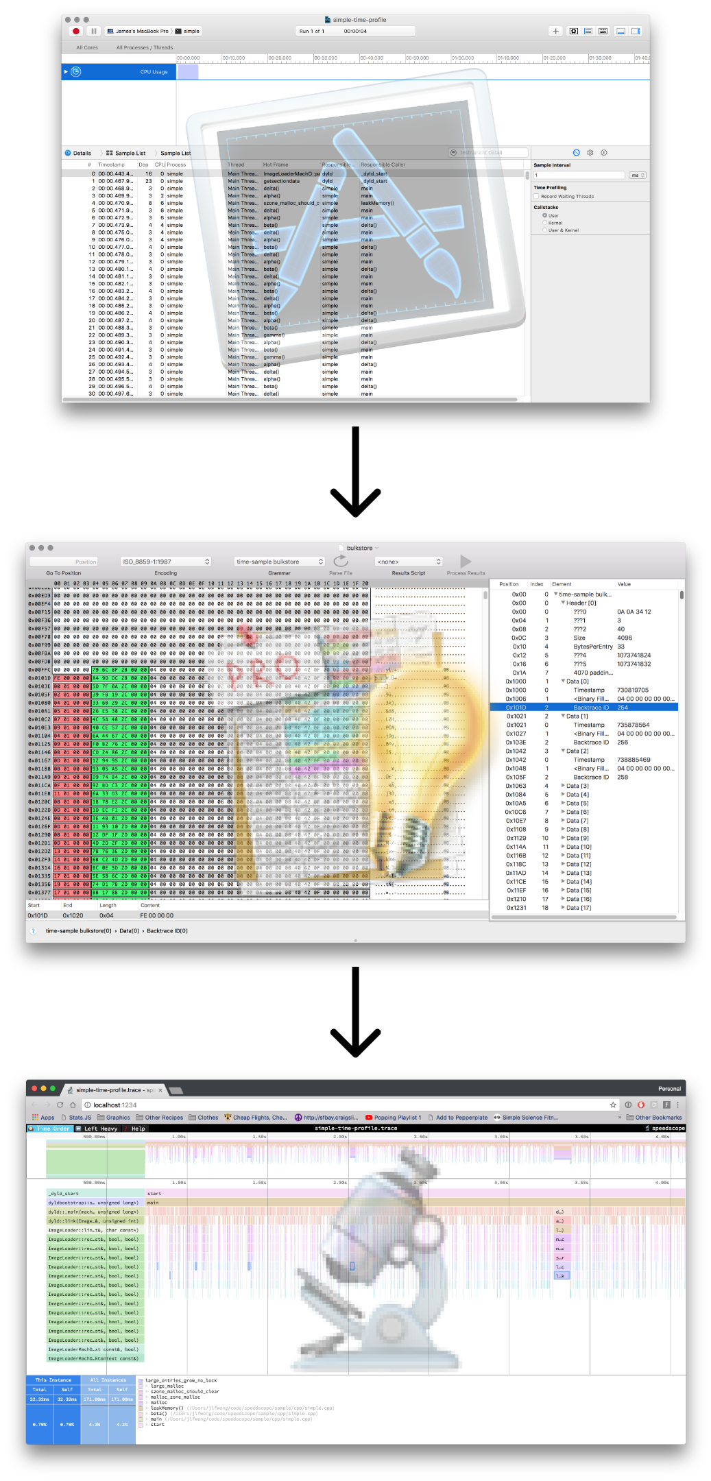
Over the last few months, I’ve been building a performance visualization tool called speedscope. It can import CPU profile formats from a variety of sources, like Chrome, Firefox, and Brendan Gregg’s stackcollapse format.

At Figma, I work in a C++ codebase that cross-compiles to asm.js and WebAssembly to run in the browser. Occasionally, however, it’s helpful to be able to profile the native build we use for development and debugging. The tool of choice to do that on OS X is Instruments. If we can extract the right information from the files Instruments outputs, then we can construct flamecharts to help us build intuition for what’s happening while our code is executing.

Up until this point, all of the formats I’ve been importing into speedscope have been either plaintext or JSON, which lends them to easier analysis. Instruments’ .trace file format, by contrast, is a complex, multi-encoding format which seems to use several hand-rolled binary formats.

This was my first foray into complex binary file reverse engineering, and I’d like to share my process for doing it, hopefully teaching you about some tools along the way.

Disclaimer: I got stuck many times trying to understand the file format. For the sake of brevity, what’s presented here is a much smoother process than I really went. If you get stuck trying to do something similar, don’t be discouraged!

Before we dig into the file format, it will be helpful to understand what kind of data we need to extract. We’re trying to import a CPU time profile, which helps us answer the question “where is all the time going in my program?” There are many different ways to analyze runtime performance of a program, but one of the most common is to use a sampling profiler.

While the program being analyzed is running, a sampling profiler will periodically ask the running program “Hey! What are you doing RIGHT NOW?”. The program will respond with its current call stack is (or call stacks, in the case of a multithreaded program), then the profiler will record that call stack along with the current timestamp. A manual way of doing this if you don’t have a profiler is to just repeatedly pause the program in a debugger and look at the call stack.

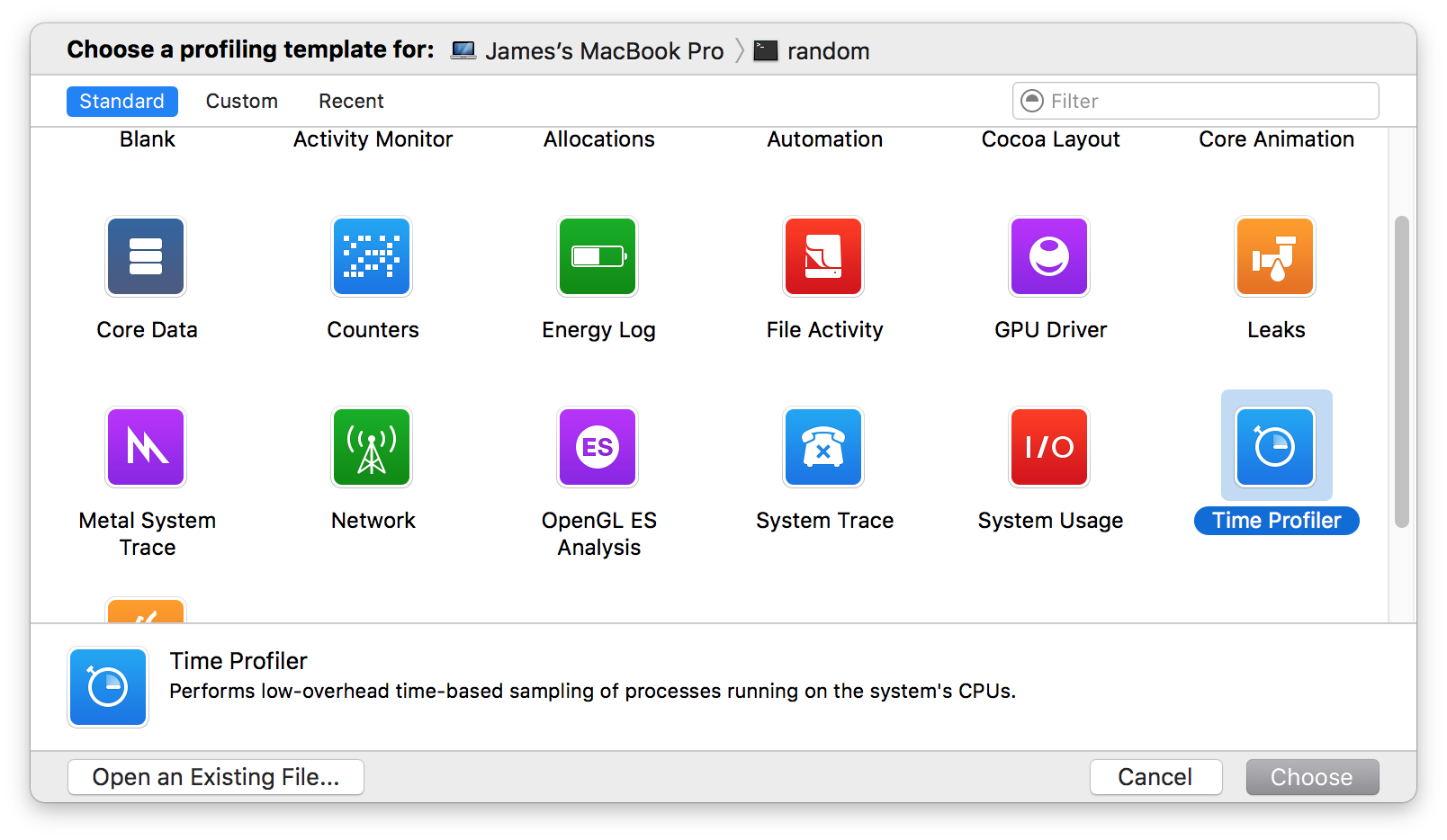
Instruments’ Time Profiler is a sampling profiler.

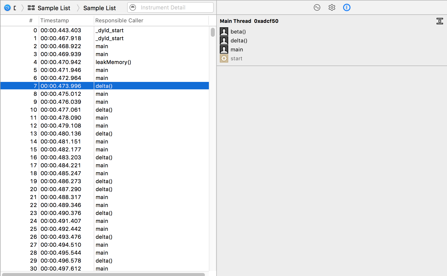
After you record a time profile in Instruments, you can see list of samples with their timestamps and associated call stacks.

This is exactly the information we want to extract: timestamps, and call stacks.

If you’d like to follow along with these steps, you can find my test file here: simple-time-profile.trace, which is a profile from Instruments 8.3.3. This is a time profile of a simple program I made specifically for analysis without any complex threading or multi-process behaviour: simple.cpp.

A good first step when trying to analyze any file is to use the unix file program.

file will try to guess the type of a file by looking at its bytes. Here are some examples:

$ file favicon-16x16.png
favicon-16x16.png: PNG image data, 16 x 16, 8-bit colormap, non-interlaced
$ file favicon.ico
favicon.ico: MS Windows icon resource - 3 icons, 48x48, 256-colors
$ file README.md
README.md: UTF-8 Unicode English text, with very long lines
$ file /Applications/Google\ Chrome.app/Contents/MacOS/Google\ Chrome
/Applications/Google Chrome.app/Contents/MacOS/Google Chrome: Mach-O 64-bit executable x86_64

So let’s see what file has to say about our .trace file.

$ file simple-time-profile.trace
simple-time-profile.trace: directory

Interesting! So the Instruments .trace file format isn’t a single file, but a directory.

macOS has a concept of a bundle, which is effectively a directory that can act like a file. This allows many different file formats to be packaged together into a single entity. Other file formats like Java’s .jar and Microsoft Office’s .docx. accomplish similar goals by grouping many different file formats together in a zip compressed archive (they’re literally just zip archives with different file extensions).

With that in mind, let’s take a look at the directory structure using the tree command, installed on my Mac via brew install tree.

$ tree -L 4 simple-time-profile.trace
simple-time-profile.trace
├── Trace1.run
│   ├── RunIssues.storedata
│   ├── RunIssues.storedata-shm
│   └── RunIssues.storedata-wal
├── corespace
│   ├── MANIFEST.plist
│   ├── currentRun
│   │   └── core
│   │       ├── extensions
│   │       ├── stores
│   │       └── uniquing
│   └── run1
│       └── core
│           ├── core-config
│           ├── extensions
│           ├── stores
│           ├── table-manager
│           └── uniquing
├── form.template
├── instrument_data
│   └── 20202640-0B46-4698-ADAD-DF54B3ABE816
│       └── run_data
│           └── 1.run.zip
├── open.creq
└── shared_data
    └── 1.run

…okay then! There’s a lot going on in here, and it’s not clear where we should be looking for the data we’re interested in.

Strings tend to be the easiest kind of data to find. In this case, we expect to find the function names of the program somewhere in the profile. Here’s the main function of the program we profiled:

intmain(intargc,char*argv[]){while(true){alpha();beta();gamma();delta();}return0;}

If we’re lucky, we’ll find the string gamma somewhere in plaintext in the .trace bundle. If the data were compressed, we might not be so lucky.

$ grep -r gamma simple-time-profile.trace
Binary file simple-time-profile.trace/form.template matches

Cool, so form.template contains the string gamma in it somewhere. Let’s see what kind of file this is.

$ file simple-time-profile.trace/form.template
simple-time-profile.trace/form.template: Apple binary property list

So what’s this Apple binary property list thing?

From a Google search, I found an article about converting binary plists, which references a tool called plutil for analyzing and manipulating the contents of binary plists. plutil -p seems especially promising as a way of printing plists in a human readable format.

$ plutil -p simple-time-profile.trace/form.template
{
  "$version" => 100000
  "$objects" => [
    0 => "$null"
    1 => "rsrc://Template - samplertemplate"
    2 => {
      "NSString" => <CFKeyedArchiverUID ...>{value = 3}
      "NSDelegate" => <CFKeyedArchiverUID ...>{value = 0}
      "NSAttributes" => <CFKeyedArchiverUID ...>{value = 5}
      "$class" => <CFKeyedArchiverUID ...>{value = 11}
    }
    ...(many more entries here, excluded for brvity)
  ]
  "$archiver" => "NSKeyedArchiver"
  "$top" => {
    "com.apple.xray.owner.template" => <CFKeyedArchiverUID ...>{value = 12}
    "com.apple.xray.instrument.command" => <CFKeyedArchiverUID ...>{value = 234}
    "$1" => <CFKeyedArchiverUID ...>{value = 163}
    "cliTargetDevice" => <CFKeyedArchiverUID ...>{value = 0}
    "com.apple.xray.owner.template.description" => <CFKeyedArchiverUID ...>{value = 2}
    "$2" => <CFKeyedArchiverUID ...>{value = 164}
    "com.apple.xray.owner.template.version" => 2.1
    "com.apple.xray.owner.template.iconURL" => <CFKeyedArchiverUID ...>{value = 1}
    "$0" => <CFKeyedArchiverUID ...>{value = 141}
    "com.apple.xray.run.data" => <CFKeyedArchiverUID ...>{value = 247}
  }
}

I wasn’t familiar with many Mac APIs, so the best I could do was just Google search some of the terms in here. CFKeyedArchiverUID shows up a lot here, and that sounds related to NSKeyedArchiver.

A Google search tells me that NSKeyedArchiver is an Apple-provided API for serialization and deserialization of object graphs into files. If we can figure out how to reconstruct the object graph that was serialized into this, this might be instrumental in extracting the data we need!

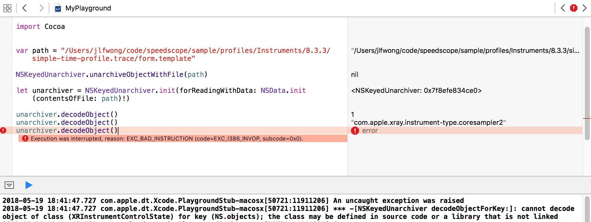
A convenient way to explore Cocoa APIs is inside of an XCode Playground. Inside of a playground, I was able to construct an NSKeyedUnarchiver and start to pull data out of it, but I quickly ran into problems:

In particular, we have this error:

cannot decode object of class (XRInstrumentControlState) for key (NS.objects);
the class may be defined in source code or a library that is not linked

Unsurprisingly, in order to decode the objects stored within a keyed archive, you need to have access to the classes that were used to encode them. In this case, we don’t have the class XRInstrumentControlState, so the archiver has no idea how to decode it!

We could probably work around this limitation by subclassing NSKeyedUnarchiver and overriding the method which decides which class to decode to based on the class name, but I ultimately want to be able to read these files via JavaScript in the browser where I won’t have access to the Cocoa APIs. Given that, it would be helpful to understand how the serialization format works more directly.

To be able to extract data from this file, we’ll both need to be able to do the same thing as plutil -p is doing above, and also do the same thing as a NSKeyedUnarchiver would be doing in reconstructing the object graph from the plist file.

Thankfully, parsing binary plists is a problem that many others have encountered in the past. Here are some binary plists parsers in a variety of languages:

Ultimately, I ended up making minor modifications to a binary plist parser that we use at Figma for Sketch import, which you can now find in the speedscope repository in instruments.ts.

Also helpfully, other people have done analysis on how NSKeyedArchiver serializes its data into a property list. This blogpost by mac4n6, for example, explores an example of how an object graph can be reconstructed from the property list. It ends up being a relatively straightforward process of replacing numerical IDs with their corresponding entries in the $object lookup table.

After these replacements are completed, objects will have a property indicating what class they were serialized from. Many common datatypes have consistent serialization formats that we can use to construct a useful representation of the original object.

This too ends up being a task that surprisingly many people have been interested in solving, and have also kindly release source code to solve:

You can see examples of these in patternMatchObjectiveC in the speedscope source code.

There are datatypes in simple-time-profile.trace/form.template, however, that are specific to Instruments. When we’re trying to reconstruct an object from an NSKeyedArchive, we’re given a $classname variable. If we collect all the Instruments-specific classnames and print them out, we’re left with this:

[
  "XRRecordingOptions",
  "XRContext",
  "XRAnalysisCoreDetailNode",
  "XRAnalysisCoreTableQuery",
  "XRMainWindowUIState",
  "XRInstrumentControlState",
  "XRRunListData",
  "XRIntKeyedDictionary",
  "PFTPersistentSymbols",
  "XRArchitecture",
  "PFTSymbolData",
  "PFTOwnerData",
  "XRCore",
  "XRThread",
  "XRBacktraceTypeAdapter"
]

Stepping back, what we’re trying to figure out here is where the function names and file locations are stored within this file. From surveying the list of Instruments specific classes above, PFTSymbolData seems like a good candidate to contain this information.

A google search of PFTSymbolData yields this github page showing a reverse-engineered header file from XCode!

@interface PFTSymbolData : NSObject <NSCoding, CommonSymbol, XRUIStackFrame, NSCopying>
{
    NSString *sourcePath;
    struct XRLineNumData *addressData;
    int numAddresses;
    int addressesCapacity;
    BOOL _missingSymbolName;
    struct _CSRange symbolRange;
    unsigned int fTypeFlags;
    PFTOwnerData *ownerData;
    NSMutableArray *inlinedInstances;
    NSString *symbolName;
}

These headers were extracted using class-dump. This was pretty lucky — it just so happens that someone has dumped all of the headers in XCode and put it up in a GitHub repository.

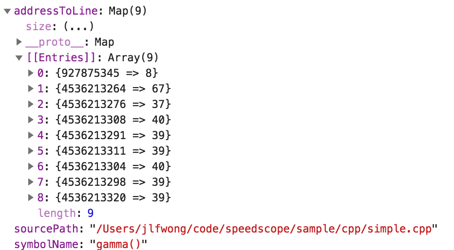
Using the header as a reference and inspecting the data, I was able to reconstruct a semantically useful representation of PFTSymbolData

You can see the relevant code in readInstrumentsKeyedArchive.

Now we have the symbol table, but we still need the list of samples!

I was hoping that all of the information I was interested in would be in a single file within the .trace bundle, but it turns out we aren’t so lucky.

The next thing I’m looking for is the list of samples collected during instrumentation. Each sample contains a timestamp, so I expect them to be stored as a table of numbers. But I wasn’t even sure what numbers I should be looking for, because I’m not sure how the timestamps are stored. The timestamps could be stored as absolute values since unix epoch, or could be stored as relative to the previous sample, or relative to the start of the profile, and could be stored as floating point values or integers, and those integers might be big endian or small endian.

Overall, I wasn’t really sure how to find data when I didn’t know any values that would definitely be in the data table, so I had a different idea for an approach. I recorded a longer profile, then went looking for big files! I figured that as profiles got longer, the data storing the list of samples should get bigger.

To find potential files of interest, I ran the following unix pipeline:

$ find . -type f | xargs du | sort -n | tail -n 10
152     ./corespace/run1/core/stores/indexed-store-9/spindex.0
168     ./corespace/run1/core/stores/indexed-store-12/spindex.0
296     ./corespace/run1/core/stores/indexed-store-3/bulkstore
600     ./form.template
808     ./corespace/run1/core/stores/indexed-store-9/bulkstore
1064    ./corespace/run1/core/stores/indexed-store-12/bulkstore
2048    ./corespace/run1/core/uniquing/arrayUniquer/integeruniquer.data
2048    ./corespace/run1/core/uniquing/typedArrayUniquer/integeruniquer.data
20480   ./corespace/currentRun/core/uniquing/arrayUniquer/integeruniquer.data
20480   ./corespace/currentRun/core/uniquing/typedArrayUniquer/integeruniquer.data

Let’s break down this pipeline.

• find . -type f finds all files in the current directory, printing them one per line (find man page)
• xargs du runs du to find file size using the list piped to it as arguments using xargs. We could alternatively do du $(find . -type f). (xargs man page, du man page)
• sort -n numerically sorts the results in ascending order (sort man page`)
• tail -n 10 takes the last 10 lines of output (tail man page)

We can extend this command to tell us the file type of each of these files:

$ find . -type f | xargs du | sort -n | tail -n 10 | cut -f2 | xargs file
./corespace/run1/core/stores/indexed-store-9/spindex.0:                     data
./corespace/run1/core/stores/indexed-store-12/spindex.0:                    data
./corespace/run1/core/stores/indexed-store-3/bulkstore:                     data
./form.template:                                                            Apple binary property list
./corespace/run1/core/stores/indexed-store-9/bulkstore:                     data
./corespace/run1/core/stores/indexed-store-12/bulkstore:                    data
./corespace/run1/core/uniquing/arrayUniquer/integeruniquer.data:            data
./corespace/run1/core/uniquing/typedArrayUniquer/integeruniquer.data:       data
./corespace/currentRun/core/uniquing/arrayUniquer/integeruniquer.data:      data
./corespace/currentRun/core/uniquing/typedArrayUniquer/integeruniquer.data: data

The cut command can be used to extract columns of data from a plaintext table. In this case cut -f2 selects only the second column of the data. We then run the file command on each resulting file. (cut man page)

A file type of data isn’t very informative, so we’ll have to start examining the binary contents to figure out the format ourselves.

xxd is a tool for taking a “hex dump” of a binary file (xxd man page). A hex dump of a binary file is a representation of a file displaying each byte of the file as a hexadecimal pair.

$ echo "hello" | xxd
00000000: 6865 6c6c 6f0a                           hello.

The output here shows the offset (00000000:), the hex represenation of the bytes in the file (6865 6c6c 6f0a) and the corresponding ASCII interpretation of those bytes (hello.), with . being used in place of unprintable characters. The . in this case corresponds to the byte 0a which in turn corresponds to the ASCII \n character emitted by echo.

Here’s another example using printf to emit 3 bytes with no printable representations.

$ printf "\1\2\3" | xxd
00000000: 0102 03                                  ...

Let’s use this to explore the biggest file we found.

$ xxd corespace/currentRun/core/uniquing/typedArrayUniquer/integeruniquer.data | head -n 10
00000000: 6745 2301 7e33 0a00 0100 0000 0000 0000  gE#.~3..........
00000010: 0100 0000 0000 0000 0000 0000 0000 0000  ................
00000020: 0000 0000 0000 0000 0000 0000 0000 0000  ................
00000030: 0000 0000 0000 0000 0000 0000 0000 0000  ................
00000040: 0000 0000 0000 0000 0000 0000 0000 0000  ................
00000050: 0000 0000 0000 0000 0000 0000 0000 0000  ................
00000060: 0000 0000 0000 0000 0000 0000 0000 0000  ................
00000070: 0000 0000 0000 0000 0000 0000 0000 0000  ................
00000080: 0000 0000 0000 0000 0000 0000 0000 0000  ................
00000090: 0000 0000 0000 0000 0000 0000 0000 0000  ................

Hmm. It seems like there’s a lot of data in this file that’s all zero’d out. The sample list can’t possibly be all zeros, so we’d rather just look for bits that aren’t zero’d out. The -a flag of xxd can be of help in this situation.

       -a | -autoskip
              toggle autoskip: A single '*' replaces nul-lines.  Default off.


$ xxd -a ./corespace/currentRun/core/uniquing/typedArrayUniquer/integeruniquer.data
00000000: 6745 2301 7e33 0a00 0100 0000 0000 0000  gE#.~3..........
00000010: 0100 0000 0000 0000 0000 0000 0000 0000  ................
00000020: 0000 0000 0000 0000 0000 0000 0000 0000  ................
*
009ffff0: 0000 0000 0000 0000 0000 0000 0000 0000  ................

Welp. It doesn’t seem like this file actually contains much useful data. Let’s re-sort our list of files, this time sorting by the number of non-null lines.

$ for f in $(find . -type f); do echo "$(xxd -a $f | wc -l) $f"; done | sort -n | tail -n 10
    1337 ./corespace/currentRun/core/extensions/com.apple.dt.instruments.ktrace.dtac/knowledge-rules-0.clp
    1337 ./corespace/run1/core/extensions/com.apple.dt.instruments.ktrace.dtac/knowledge-rules-0.clp
    2232 ./corespace/currentRun/core/extensions/com.apple.dt.instruments.poi.dtac/binding-rules.clp
    2232 ./corespace/run1/core/extensions/com.apple.dt.instruments.poi.dtac/binding-rules.clp
    2391 ./corespace/run1/core/uniquing/arrayUniquer/integeruniquer.data
    2524 ./corespace/run1/core/stores/indexed-store-12/spindex.0
    2736 ./corespace/run1/core/stores/indexed-store-9/spindex.0
    5148 ./corespace/run1/core/stores/indexed-store-9/bulkstore
    6793 ./corespace/run1/core/stores/indexed-store-12/bulkstore
   18091 ./form.template

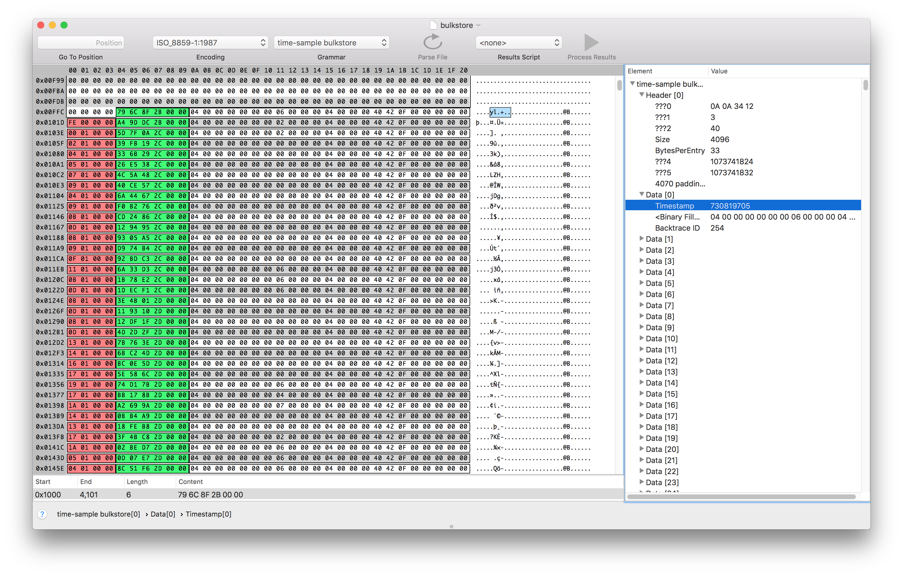
We already know what form.template is, so we’ll start with the second largest. If we look at indexed-store-12/bulkestore, it looks like there might be some useful data in there, starting at offset 0x1000.

$ xxd -a ./corespace/run1/core/stores/indexed-store-12/bulkstore | head -n 20
00000000: 0a0a 3412 0300 0000 2800 0000 0010 0000  ..4.....(.......
00000010: 2100 0000 0040 0800 0040 0000 0000 0000  !....@...@......
00000020: 0000 0000 0000 0000 0000 0000 0000 0000  ................
*
00001000: 796c 8f2b 0000 0400 0000 0000 0006 0000  yl.+............
00001010: 0004 0000 0040 420f 0000 0000 00fe 0000  .....@B.........
00001020: 00a4 9ddc 2b00 0004 0000 0000 0000 0200  ....+...........
00001030: 0000 0400 0000 4042 0f00 0000 0000 0001  ......@B........
00001040: 0000 5d7f 0a2c 0000 0400 0000 0000 0002  ..]..,..........
00001050: 0000 0004 0000 0040 420f 0000 0000 0002  .......@B.......
00001060: 0100 0039 fb19 2c00 0004 0000 0000 0000  ...9..,.........
00001070: 0000 0000 0400 0000 4042 0f00 0000 0000  ........@B......
00001080: 0401 0000 336b 292c 0000 0400 0000 0000  ....3k),........
00001090: 0000 0000 0004 0000 0040 420f 0000 0000  .........@B.....
000010a0: 0005 0100 0026 e538 2c00 0004 0000 0000  .....&.8,.......
000010b0: 0000 0000 0000 0400 0000 4042 0f00 0000  ..........@B....
000010c0: 0000 0701 0000 4c5a 482c 0000 0400 0000  ......LZH,......
000010d0: 0000 0000 0000 0004 0000 0040 420f 0000  ...........@B...
000010e0: 0000 0009 0100 0040 ce57 2c00 0004 0000  .......@.W,.....
000010f0: 0000 0000 0000 0000 0400 0000 4042 0f00  ............@B..

The @B in the right column, while not obviously semantically meaningful, seems to repeat at a regular interval. Maybe if can figure out that regular interval, we’ll be able to guess what the structure of the data is. We can try guessing different intervals by using the -c argument of xxd, and try changing the byte grouping using the -g argument.

      -c cols | -cols cols
              format <cols> octets per line. Default 16 (-i: 12, -ps: 30, -b: 6).

     -g bytes | -groupsize bytes
              separate the output of every <bytes> bytes (two hex characters or eight bit-digits each) by a whitespace.  Specify -g 0 to suppress grouping.

We seem to get alignment between the repeated values when we group data into chunks of 33:

$ xxd -a -c 33 -g0 ./corespace/run1/core/stores/indexed-store-12/bulkstore | cut -d' ' -f2 | head -n 10
0a0a34120300000028000000001000002100000000400800004000000000000000
000000000000000000000000000000000000000000000000000000000000000000
*
00000000796c8f2b000004000000000000060000000400000040420f0000000000
fe000000a49ddc2b000004000000000000020000000400000040420f0000000000
000100005d7f0a2c000004000000000000020000000400000040420f0000000000
0201000039fb192c000004000000000000000000000400000040420f0000000000
04010000336b292c000004000000000000000000000400000040420f0000000000
0501000026e5382c000004000000000000000000000400000040420f0000000000
070100004c5a482c000004000000000000000000000400000040420f0000000000

Sweet! This suggests that this file format uses 33 bytes per entry, and hopefully each of those entries corresponds to one sample in the profile.

Looking around in the directory which contains this bulkstore, we find a helpful sounding file called schema.xml:

$ cat ./corespace/run1/core/stores/indexed-store-12/schema.xml<schema name="time-profile" topology="XRT50_C22_TypeID"><column engineeringType="XRSampleTimestampTypeID" engineeringName="Sample Time" mnemonic="time" topologyField="XRTraceRelativeTimestampFieldID"></column><column engineeringType="XRThreadTypeID" engineeringName="Thread" mnemonic="thread" topologyField="XRCategory1FieldID"></column><column engineeringType="XRProcessTypeID" engineeringName="Process" mnemonic="process"></column><column engineeringType="XRCPUCoreTypeID" engineeringName="Core" mnemonic="core"></column><column engineeringType="XRThreadStateTypeID" engineeringName="State" mnemonic="thread-state"></column><column engineeringType="XRTimeSampleWeightTypeID" engineeringName="Weight" mnemonic="weight"></column><column engineeringType="XRBacktraceTypeID" engineeringName="Stack" mnemonic="stack"></column></schema>

Alright, this is looking pretty good! XRSampleTimestampTypeID and XRBacktraceTypeID seem particularly relevant.

The next step is to figure out how these 33 byte entries map onto the fields in schema.xml.

So far in this exploration, all of the tools I’ve been using come standard on most unix installations, and all are free and open source. While I certainly could have figured this out end-to-end using only tools in that category, my friend Peter Sobot introduced me to a tool that made this process much easier.

Synalyze It! is a hex editor and binary analysis tool for OS X. There’s a Windows & Linux version called Hexinator. These tools let you make guesses about the structure of file formats (e.g. “I think this file is a list of structs, each of which is 20 bytes, where the first 4 bytes are an unsigned int, and the last 16 bytes are a fixed-length ascii string”), then parse the file based on that guess and display in both a colorized view of the hex dump and in an expandable tree view. This let me guess-and-check several hypotheses about what the structure of the file.

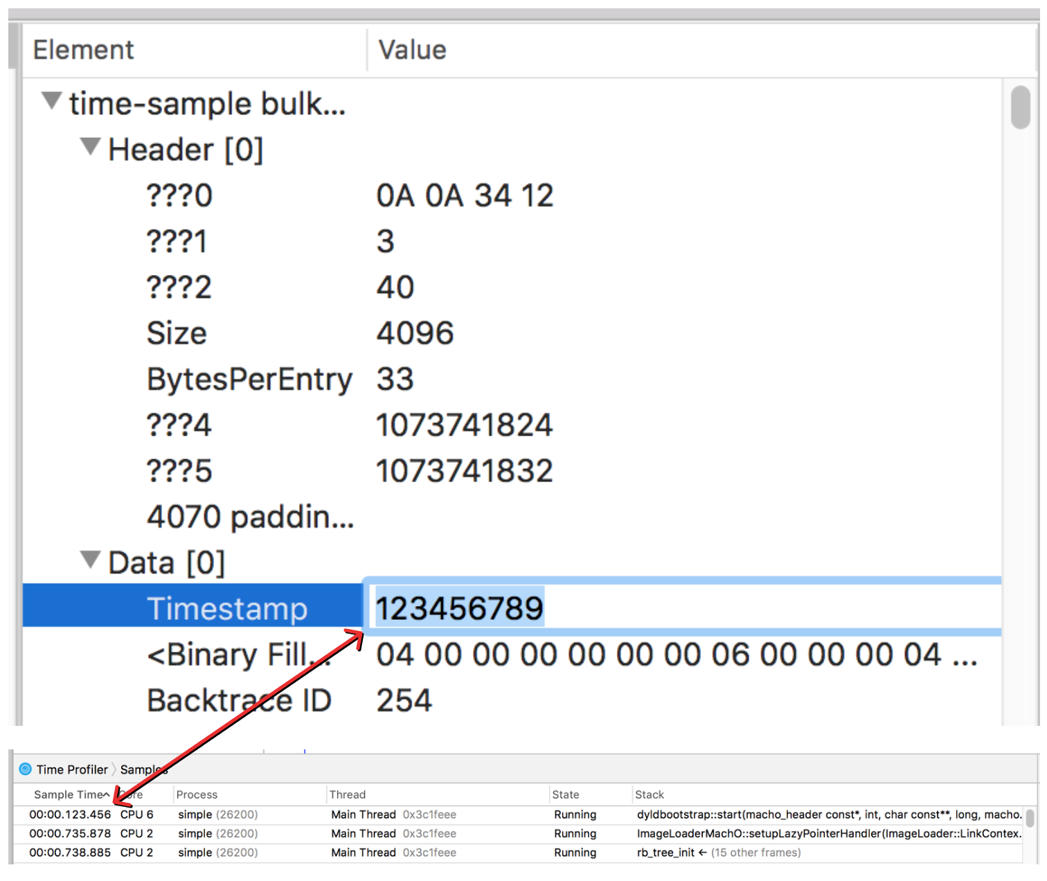
Eventually I was able to guess the length and offsets of the fields I was interested in. Synalyze It! helps you visually parse the information by setting colors for different fields. Here, I’ve set the sample timestamp to be green, and the backtrace ID to be red.

From looking at the values of the sample time and comparing them with what Instruments was displaying, I was able to infer that the values represented the number of nanoseconds since the profile started as a six byte unsigned integer. I was able to verify this by editing the binary file and then re-opening it in instruments.

Sweet! So that answers the question of where the sample information is stored, and we know how to interpret the timestamp data. But we still don’t quite know how to turn the backtrace ID into a stack trace.

To try to find the stacks, we can see if the memory addresses identified as part of the symbol table show up anywhere outside of the form.template binary plist.

Here’s the same symbol data from earlier.

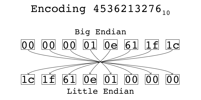
So let’s see if we can find one of these addresses referenced somewhere else in the .trace bundle. We’ll look for the third address in that list, 4536213276.

As a first attempt, it’s possible that the number is written as a string.

$ grep -a -R -l '4536213276' .

No results. Well, that was kind of a long shot. Let’s try the more plausible idea of searching for a binary encoding of this number.

There are two standard ways of encoding multi-byte integers into a byte stream. One is called “little endian” and the other is called “big endian”. In little endian, you place the least significant byte first. In big endian, you place the most significant byte first. Using python’s struct standard library, we can see what each of these representations look like.

The number is too big to fit in a 32 bit integer, so it’s probably a 64 bit integer, which would make sense if it’s a memory address that has to support 64 bit addresses.

$ python -c 'import struct, sys; sys.stdout.write(struct.pack(">Q", 4536213276));' | xxd
00000000: 0000 0001 0e61 1f1c                      .....a..
$ python -c 'import struct, sys; sys.stdout.write(struct.pack("<Q", 4536213276));' | xxd
00000000: 1c1f 610e 0100 0000                      ..a.....

>Q instructs struct.pack to encode the number as a big endian 64 bit unsigned integer, and <Q corresponds to a little endian 64 bit unsigned integer.

If you split up the bytes, you can see it’s the same bytes in both encodings, just in reverse order:

Now we can use a little python program to search for files with the value we care about.

$ cat search.py
import os, glob, struct

addr = 4536213276
little = struct.pack('<Q', addr)
big = struct.pack('>Q', addr)

for (dirpath, dirnames, filenames) in os.walk('.'):
  for f in filenames:
    path = os.path.join(dirpath, f)
    contents = open(path).read()
    if little in contents:
      print 'Found little in %s' % path
    elif big in contents:
      print 'Found big in %s' % path
$ python search.py
Found big in ./form.template
Found little in ./corespace/run1/core/uniquing/arrayUniquer/integeruniquer.data

Sweet! The value is in two places: one little endian, one big endian. The form.template one we already knew about — that’s where we found this address in the first place. The second location in integeruniquer.data is one we haven’t explored. It also was one of the files we found when searching for files with large amounts of non-zero data in them.

After fumbling around in this file with Synalyze It! for a while, I discovered that file is aptly named, and contains arrays of integers packed as a 32 bit length followed by a list of 64 bit integers.

So integeruniquer.data contains an array of arrays of 64 bit integers. Neat! It seems like each 64 bit int is either a memory address or an index into the array of arrays. This was the last piece of the puzzle we need to parse the profiles.

So overall, the final process looks like this:

1. Find the list of samples by finding a bulkstore file adjacent to a schema.xml which contains the string <schema name="time-profile".
2. Extract a list of (timestamp, backtraceID) tuples from the bulkstore
3. Using the backtraceID as an index into the array represented by arrayUniquer/integeruniquer.data, convert the list of (timestamp, backtraceID) tuples into a list of (timestamp, address[]) tuples
4. Parse the form.template binary plist and extract the symbol data from PFTSymbolData from the resulting NSKeyedArchive. Convert this into a mapping from address to (function name, file path) pairs.
5. Using the address → (function name, file path) mapping in conjunction with the (timestamp address[]) tuple list, construct a list of (timestamp, (function name, file path)[]) tuples. This is the final information needed to construct a flamegraph!

Phew! That was a lot of digging for what ultimately ends up being a relatively straightforward data extraction. You can find the implementation in importFromInstrumentsTrace in the source for speedscope on GitHub.

If you do get the chance to give speedscope a try, please tweet @jlfwong and let me know what you think 🙂.

Thanks toPeter Sobot,Ryan Kaplan, andRudi Chenfor providing feedback on the draft of this post.

When PagerDuty was founded, development speed was of the essence—so it should be no surprise when we reveal that Rails was the initial sole bit of technology we ran on. Soon, limitations caused the early team to look around and Scala was adopted to help us scale up.

However, there’s a huge gap between Scala and Ruby, including how the languages look and what the communities find important; in short, how everything feels. The Ruby community, and especially the Rails subcommunity, puts a huge value on the developer experience over pretty much anything else. Scala, on the other hand, has more academic and formalistic roots and tries to convince its users that correctness trumps, well, pretty much anything.

It nagged me and it looked like we had a gap in our tech stack that was hard to reconcile. Scala wasn’t likely to going to power our main site, and though we needed better performance and better scalability than Ruby and Rails could deliver, there was a very large gap and switching was cumbersome. There was also little love for the initial Scala codebase, as it quickly became apparent that writing clean and maintainable Scala code was hard and some technology choices made scaling more difficult than anticipated.

When thinking about these issues in 2015, I let myself be guided by an old Extreme Programming practice, that of the System Metaphor. Given that I did some work in the telecommunications world, it wasn’t too far-fetched to look at PagerDuty like some sort of advanced (telco) switch: stuff comes in, rules and logic route and change it, and stuff goes out. As with any analogy, you can stretch it as far as you want (look at an incident as an open circuit), but for me, just squinting a bit and realizing that it was a workable metaphor was enough.

If you say “telecom” and “programming language,” you say “Erlang.” I looked at Erlang before but the language never appealed to me, and in the past, it never really hit the sweet spot in terms of the kinds of systems I was working on. This time, however, the “sweet spot” part seemed to hold, but still—a language that was based on Prolog, that got a lot of things backward (like mixing up what’s uppercased and what’s lowercased), felt like C with header files … that would be a hard sell.

So I parked that idea, went back to work, and forgot about it until I stumbled upon Elixir a month or two later. Now this was interesting! Someone with Ruby/Rails street cred went off, built a language on top of Erlang’s Virtual Machine: One that was modern, fast, very high level, had Lisp/Scheme-style macros, and still professed to be nice to users (rather than Ph.D. students).

Needless to say, it immediately scored the top spot on my “languages to learn this year” list and I started working through documentation, example code, etc. What was promised, held up—it performed above expectations both in execution as well as in development speed. And what’s more, developing in Elixir was sheer fun.

After getting my feet wet and becoming more and more convinced that this could indeed remove the need for Scala, be nicer to Ruby users, and overall make us go faster while having more fun, I started looking for the dreaded Pilot Project.

Introducing Elixir

Introducing languages is tricky. There’s a large cost involved with the introduction of new programming languages, although people rarely account for that. So you need to be sure. And the only way to be sure is, somewhat paradoxically, to get started and see what happens. As such, a pilot needs to have skin in the game, be mission-critical, and be complex yet limited enough that you can pull the plug and rewrite everything in one of your old languages.

For my team, the opportunity came when we wanted to have a “Rails-native” way to talk to Kafka transactionally. In order to ease the ramp-up for the MySQL-transaction-heavy Rails app, we wanted to build a system that basically scraped a database table for Kafka messages and sent it to Kafka. Though we knew this wasn’t really the best way to interact with Kafka, it did allow us to simply emit Kafka messages as part of the current ActiveRecord transaction. That made it really easy to enhance existing code with Kafka side effects and reason about what would happen on rollbacks, etc.

We opted for this project as our Elixir pilot—it was high value and the first planned Kafka messages would be on our critical notification path, but it was still very self-contained and would have been relatively easy to redo in Scala if the project failed. It doesn’t often happen that you stumble upon pretty much the perfect candidate for a new language pilot, but there it was. We jumped into the deep and came out several weeks later with a new service that required a lot of tuning and shaping, but Elixir never got in the way of that.

Needless to say, this didn’t sway the whole company to “Nice, let’s drop everything and rewrite all we have in Elixir,” but this was an important first step. We started evangelizing, helped incubate a couple more projects in other teams, and slowly grew the language’s footprint. We also tried to hire people who liked Elixir, hosted a lot of Toronto Elixir meetups to get in touch with the local community, and—slowly but steadily—team after team started adopting the language. Today, we have a good mix of teams that are fully on Elixir, teams that are ramping up, and teams who are still waiting for the first project that will allow them to say, “We’ll do this one in Elixir.”

Elixir has been mostly selling itself: it works, it sits on a rock-solid platform, code is very understandable as the community has a healthy aversion towards the sort of “magic” that makes Rails tick, and it’s quite simple to pick up as it has a small surface area. By now, it’s pretty unlikely that anything that flows through PagerDuty is not going to be touched by Elixir code. This year, we’re betting big on it by lifting some major pieces of functionality out of their legacy stacks and into Elixir, and there are zero doubts on whether Elixir will be able to handle the sort of traffic that PagerDuty is dealing with in 2018. From initial hunch through pilot into full-scale production, it’s been a pretty gentle ride and some of us are secretly hoping that one day, we’ll only have to deal with Elixir code.

An article on Elixir would not be complete without a shout out to the community’s leadership, starting with Elixir inventor José Valim, whom I largely credit for the language’s culture. Elixir comes with one of the nicest and most helpful communities around, and whether on Slack, on the Elixir Forum, or on other channels like Stack Overflow and IRC, people are polite, helpful, and cooperative. Debates are short and few, and the speed of progress is amazing. That alone makes Elixir worth a try.

Want to chat more about Elixir? PagerDuty engineers can usually be found at the San Francisco and Toronto meetups. And if you’re interested in joining PagerDuty, we’re always looking for great talent—check out our careers page for current open roles.

Blot is a blogging platform with no interface. It creates a special folder in your Dropbox and publishes files you put inside. The point of all this — the reason Blot exists — is so you can use your favorite tools to create whatever you publish.

Blot automatically creates blog posts from Text and Markdown,  Word Documents,  Images,  Bookmarks and  HTML. Just put the files inside your blog’s folder and Blot does the rest.

Blot comes with seven templates. They’re easy to customize, lightweight and designed to fit both small and large screens. You can also develop your own template from scratch.

A blog costs $20 per year. The annual fee pays for the servers which host your blog. It also covers the cost of providing support. Here’s a handful of the websites hosted on Blot:

For over a hundred years the analog dog wagged the digital tail. The effort to extend the reach of our senses – sight, hearing, even (after a manner of speaking) touch, drove engineers and scientists to search for better components for telegraph, telephone, radio and radar equipment. It was a happy accident that this also opened the door to new kinds of digital machines.¹ I set out to tell the story of this repeated exaptation, whereby telecommunications engineers supplied the raw materials of the first digital computers, and sometimes even designed and built such computers themselves.

By the 1960s, however, this fruitful relationship came to a close, and so too does my story. The makers of digital equipment no longer had any need to look outward to the world of the telegraph, telephone, and radio for new and improved switches, because the transistor itself provided a seemingly inexhaustible vein of improvements to mine. Year after year, they dug deeper and deeper, always finding ways to exponentially increase speed and reduce costs.

None of this, however, would have happened, if the invention of the transistor had stopped with Bardeen and Brattain.

A Slow Start

The popular press did not react to Bell Labs’ announcement of the transistor with great enthusiasm. On July 1, 1948, The New York Times gave it three paragraphs at the bottom of their “The News of Radio” bulletin. The notice appeared after several other announcements evidently deemed more significant: touting, for example, the one-hour “Waltz Time” broadcast coming to NBC. Hindsight tempts us to mock, or even scold, the ignorance of the anonymous authors – how did they fail to recognize the world-shaking event that had just transpired?

But hindsight distorts, amplifying the few signals that we now know to be significant,  though at the time they were lost in a sea of noise. The transistor of 1948 was very different from the transistors in the computer on which you are reading this². So different that, despite their common name and the unbroken line of ancestry that connects them, they should be considered a different species of thing, if not a different genus. They share neither material composition, nor structural form, nor functional principles; not to mention their tremendous difference in size. Only by being reinvented again and again did the clunky device constructed by Bardeen and Brattain become capable of transforming the world and the way we live in it.

In truth, the germanium point-contact transistor deserved no more attention than it got. It suffered from a number of defects relative to its vacuum tube cousin. To be sure, it was rather smaller than even the most compact tube. Its lack of a heated filament meant it generated less heat, consumed less power, would not burn out, and required no warming up before it could be used.

But the accumulation of dirt on the contact surface led to failures and undermined its potential for longer life; it produced a noisier signal; worked only at low power and in a narrow frequency band; failed when exposed to heat, cold or humidity; and could not be produced uniformly. A sequence of transistors all constructed in the same way by the same people would differ obnoxiously in their electrical characteristics. All of this baggage came at a retail price some eight times higher than that of a typical tube.

Not until 1952 did Bell (and other patent licensees) work out the manufacturing kinks sufficiently for point-contact transistors to see real use, and even so they never spread much beyond the hearing aid market, where price sensitivity was relatively low, and the advantages offered in battery life dominated other considerations.³

The first efforts to remake the transistor into something better and more useful, however, had already begun. In fact, they began well before the public even learned that the transistor existed.

Shockley’s Ambition

As the year 1947 came to a close, an agitated Bill Shockley took a business trip to Chicago. He had some vague ideas about how to trump Bardeen and Brattain’s recently invented transistor, but he had not yet had the chance to develop them. And so, rather than enjoy his time off between business engagements, he spent New Year’s Eve and New Year’s Day in his hotel room, scribbling out some twenty pages of notes on his ideas. Among them was a proposal for a new kind of transistor consisting of a kind of semiconductor sandwich – a slice of p-type germanium between two pieces of n-type.

Emboldened by this ace in his back pocket, Shockley then confronted Bardeen and Brattain on his return to Murray Hill, claiming full credit for the invention of the transistor. Had it not been his field-effect idea that had sent Bardeen and Brattain scurrying off to the lab? Should not the authorship of the patent thus fall entirely to him? But Shockley’s stratagem backfired: Bell Labs patent lawyers found that an obscure inventor, Julius Lilienfeld, had patented a field-effect semiconductor amplifier almost twenty years prior, in 1930. Lilienfeld had surely never built the thing he proposed, given the state of materials science at the time, but the risk of an interference proceeding was too great – better to avoid mentioning the field effect in the patent altogether.

So, though Bell Labs would allow Shockley a generous share of the public credit, it named only Bardeen and Brattain in the patent. The damage was done, however: Shockley’s ambition destroyed his relationship with his two subordinates. Bardeen abandoned the transistor, and shifted his focus to superconductivity. He left Bell Labs in 1951. Brattain remained but refused to work with Shockley again, and insisted on being transfered to another group.

His inability to get along with others made it impossible for Shockley to rise any further at Bell Labs, and so he too jumped ship. In 1956, he returned home to Palo Alto to found his own transistor manufacturing company, Shockley Semiconductor. Before leaving for the West Coast, he left his wife Jean, while she was recovering from uterine cancer, for his soon-to-be second wife, Emmy Lanning. But of the two halves of his California dream — new company and new wife — only one would last. In 1957, Shockley’s best engineers, irritated by his management style and the direction in which he was taking the company, defected to form a new firm called Fairchild Semiconductor.

So Shockley abandoned the hollowed-out husk of his company to take a position in the electrical engineering department at Stanford. There he proceeded to alienate his colleagues (and his oldest friend, physicist Fred Seitz) with his newfound interest in dysgenics and racial hygiene – unpopular topics in the United States since the late war, especially so in academia. He delighted in stirring up controversy, riling up the media, and drawing protesters. He died in 1989, alienated from his children and his peers, attended only by his eternally devoted second wife, Emmy.

Though his own attempt at entrepreneurship had failed miserably, Shockley had cast seed onto fertile ground. The San Francisco Bay area teemed with small electronics firms and had been irrigated with funds from the federal government during the war. Fairchild Semiconductor, Shockley’s accidental offspring, itself spawned dozens of new firms, among them two names still very well-known today: Intel and Advanced Micro Devices (AMD). By the early 1970s, the area had acquired the moniker “Silicon Valley.” But wait – Bardeen and Brattain had built a germanium transistor. Where did the silicon come from?

To The Silicon Junction

The new kind of transistor that Shockley devised in his Chicago hotel had a happier destiny than that of its inventor. This was thanks to one man’s determination to grow single, pure semiconductor crystals. Gordon Teal, a physical chemist from Texas who had studied the then-useless element of germanium for his doctoral thesis, had joined Bell Labs in the thirties. After learning about the transistor, he became convinced that its reliability and power could be vastly improved by crafting it from a pure monocrystal, rather than the polycrystalline aggregates then being used. Shockley discouraged this effort, believing that it was an unnecessary waste of resources.

But Teal persevered, and succeeded, with the help of a mechanical engineer named John Little, in constructing an apparatus that pulled a tiny seed crystal from a molten bath of germanium. As the germanium cooled around the seed, it extended its crystalline structure, drawing out a continuous, and almost entirely pure, semiconductor lattice. By the spring of 1949 Teal and Little could produce crystals on demand, and tests showed that they vastly outperformed their poly-crystalline counterparts. In particular, injected minority carriers could survive inside them for one hundred microseconds or more (versus ten microseconds or less in other crystal samples).⁴

Teal could now avail himself of more resources, and recruited more men to his team, among them another physical chemist who came to Bell Labs by way of Texas, Morgan Sparks.⁵ They began altering the melt to make p-type or n-type germanium by adding pellets of the appropriate doping agents. Within another year they had refined their technique to the point that they could actually grow an n-p-n germanium sandwich right out of the melt. And it worked just as Shockley had predicted: an electrical signal on the p-type material modulated the flow of electricity between two other leads attached to the n-type slices that surrounded it.

This grown-junction transistor outclassed its point-contact predecessor in almost every dimension. Most notably they were more reliable and predictable, far less noisy (and thus more sensitive), and extremely power efficient – drawing one million times less power than a typical vacuum tube.⁶ In July 1951, Bell Labs held another press conference to announce this new creation. Before the original transistor had even gotten off the ground commercially, it had already been rendered largely irrelevant.

Yet it was still only the beginning. In 1952, General Electric (GE) announced a new process for making junction transistors called the alloy-junction method. This involved melting two pellets of indium (a p-type donor) into either side of a thin slice n-type germanium. The process was simpler and less expensive than growing junctions out of the melt, generated less resistance, and supported higher frequencies.

The following year Gordon Teal decided to return to his home state, and took a job at Texas Instruments (TI), in Dallas. Founded as Geophysical Services, Inc., a maker of oil prospecting equipment, TI branched out into electronics during the war and was now entering the transistor market under a license from Western Electric (Bell’s manufacturing arm).

Teal brought with him the newest set of skills he had developed at Bell Labs: the ability to grow and dope monocrystals of silicon. Germanium’s most obvious weakness was its sensitivity to temperature. When exposed to heat, the germanium atoms in the crystal rapidly shed free electrons, becoming more and more like a pure conductor. At around 170 degrees Farenheit, they ceased to work as transistors altogether. The military – a potential customer with little price sensitivity and a powerful need for stable, reliable and small electronic components –  was a prime target for transistor sales. But temperature-sensitive germanium would not do for many military applications, especially in aerospace equipment.

Silicon was much more stable, but this came at the price of a much higher melting point, as high as that of steel. This created great difficulties given that pure crystals were needed to make high quality transistors. The hot molten silicon would leach impurities from whatever crucible it rested in. Teal and his team at TI managed to overcome these difficulties, with the help of ultra-high purity silicon samples from DuPont. In May 1954, at an Institute of Radio Engineers conference in Dayton, Ohio, Teal demonstrated that the new silicon devices coming out of his lab continued to amplify even when immersed in hot oil.⁷

The Upstarts

At last, some seven years after the initial invention of the transistor, it could be made from the material with which it has become synonymous. As much time again would pass before transistors appeared that roughly resemble the form of those in our microprocessors and memory chips.

In 1955, Bell Labs scientists succeeded in making silicon transistors with a new doping technique – rather than adding solid dopant pellents to liquid melt, they diffused vaporized dopants into a solid semiconductor surface. By carefully controlling the temperature, pressure and duration of exposure, they achieved exactly the desired depth and amount of doping. This more precise control of the manufacturing process resulted in a more precise control over the electrical properties of the end product. Just as importantly, the diffusion technique opened the doors to batch production – one could dope a large slab of silicon all at once and then slice it up into transistors after the fact. The military provided the cash needed to offset Bell’s high up-front costs for setting up manufacturing. They wanted the new product for the ultra-high-frequency Distant Early Warning Line, a chain of arctic radar stations designed to detect Soviet bombers coming over the North Pole, and were willing to pay $100 per transistor.⁸

Doping, combined with photolithography to control the placement of the dopants, made it possible to imagine etching a complete circuit in one semiconductor wafer, an achievement which was realized independently at Fairchild Semiconductor and Texas Instruments in 1959. Fairchild’s “planar process” used the chemical deposition of metal films to connect the transistor’s electrical contacts. This obviated the need for hand wiring, simultaneously reducing costs and increasing reliability.

Finally, in 1960, two Bell Lab engineers (John Atalla and Dawon Kahng) realized Shockley’s original concept for a field-effect transistor. A thin layer of oxide on the semiconductor surface proved highly effective at suppressing the surface states, allowing the electric field from an aluminum gate to pass into the body of the silicon. This was the origin of the MOSFET (metal-oxide semiconductor field-effect transistor), which proved so amenable to miniaturization and still features in almost all computers today.⁹ Here at last, thirteen years after the initial invention of the transistor, is something recognizably like the transistor in your computer. It was simpler to make and used less power than junction transistors, but was a laggard in responding to signals. Not until the advent of large-scale integration circuits with hundreds or thousands of components on a single chip did the advantages of field-effect transistors come to the fore.

The field-effect proved to be the last major contribution by Bell Labs to the development of the transistor. The large electronics incumbents such as Bell (via Western Electric), General Electric, Sylvania, and Westinghouse developed an impressive record of semiconductor research. From 1952-1965, Bell Labs alone secured well over two hundred patents in the field. Nonetheless the commercial marketplace rapidly passed into the hands of new players like Texas Instruments, Transitron and Fairchild.

The early market for transistors was simply too small for the big incumbents to pay much attention to: roughly $18 million a year in the mid-1950s, versus over $2 billion for the electronics market as a whole. Meanwhile, though, the research labs of those same incumbents served as unwitting training facilities, where young scientists could soak up knowledge about semiconductors before moving on to sell their services to smaller firms. By the time the market for tube electronics began to decline seriously, in the mid-1960s, it was far too late for Bell, Westinghouse and the like to overtake the upstarts.¹⁰

The Computer Transistorized

There were four notable areas where transistors made significant inroads in the 1950s. The first two were hearing aids and portable radios, where lower power consumption (and thus longer battery life) trumped other considerations. The U.S. military was the third. They had high hopes for transistors as rugged and compact components in everything from field radios to ballistic rockets. But in the early years their spending on transistors was more of a bet on the future of the technology than an indication of its present value. And, finally, there was digital computing.

In the case of the computer, the severe disadvantages of vacuum tube switches were well known, so much so that many skeptics before the war had believed that an electronic computer could never be made practical. When assembled in units of thousands, tubes devoured electrical power while generating vast amounts of heat, and could be relied on only to burn out regularly. Thus the power-sipping, cool, and filament-less transistor appeared as a kind of savior to computer manufacturers. Its disadvantages as an amplifier (such as a noisier output signal) presented much less of a problem when used as a switch. The only real obstacle was cost, and that would began to fall precipitously, in due time.

All of the early American experiments in transistorized computers occurred at the intersection of the desire of the military to explore the potential of a promising new technology, and the desire of computer engineers to migrate to a new, better kind of switch.

Bell Labs built the TRADIC in 1954 for the U.S. Air Force, to see if transistors would make it possible to send a digital computer on-board a bomber, to replace analog navigation and bomb-sighting aids.  MIT’s Lincoln Laboratory, developed the TX-0 computer as part of its vast air-defense system project, in 1956. The machine used yet another transistor variant, the surface-barrier transistor, which was well suited to high-speed computing. Philco built its SOLO computer under Navy contract (but really on behalf of the National Security Agency), completing the work in 1958. (It was another surface-barrier design.)

The story in Western Europe, which was not so flush with Cold War military resources, was rather different. Machines like the Manchester Transistor Computer, Harwell CADET (another ENIAC-inspired name, obscured by mirror-writing), and Austrian Mailüfterl were side projects, using whatever resources the creators could scrape together -including first-generation point-contact transistors.

There is much jockeying among these various projects for the title of first transistorized computer. It all, of course, depends on which definitions one chooses for “first”, “transistorized,” and “computer.” We know where the story ends up in any case. The commercialization of transistorized computers followed almost immediately. Year-by-year computers of the same price grew ever more powerful while computers of the same power fell ever lower in price, in a process so seemingly inexorable that it became enshrined as a “law”, to sit alongside gravity and the conservation of matter. Shall we quibble over which was the first pebble in the avalanche?

Why Moore’s Law?

As we reach the close of our story of the switch, it is worth asking the question: What did cause this avalanche? Why does¹¹ Moore’s Law exist? There is no Moore’s Law of airplanes or vacuum cleaners, nor, for that matter, of vacuum tubes or relays.

There are two parts to the answer:

1. The logical properties of the switch as a category of artifact
2. The ability to use entirely chemical processes to make transistors

First, the essence of the switch. The properties of most artifacts must satisfy a wide variety of non-negotiable physical constraints. A passenger airplane must be able to hold up the combined weight of many people. A vacuum cleaner must be able to pull up a certain amount of dirt in a given amount of time, over a given physical area. Neither airplanes nor vacuum cleaners would be useful if reduced to nanoscale.

On the other hand, a switch – an automatic switch, one never touched by human hands – has very few physical constraints. It needs to have two distinguishable states, and it needs to be able to tell other switches like itself to change between those states. That is to say, all it needs to do is to turn on, and turn back off again. Given this, what is special about transistors? Why have other kinds of digital switch not seen such exponential improvements?

Here we come to the second fact. Transistors can be made using chemical processes with no mechanical intervention. From the beginning, the core element of transistor manufacturing was the application of chemical dopants. Then came the planar process, which removed the last mechanical step in the manufacturing process – the attachment of wires. It thus cast off the last physical constraint on miniaturization. No longer did transistors need to be large enough for fingers – or a mechanical device of any sort – to handle. Mere chemistry would do the job, at an unimaginably tiny scale: acids to etch, light to control which parts of the surface will resist the etching, and vapors to deposit dopants and metal films into the etched corridors.

Why miniaturize in the first place? Decreased size brought with it an array of pleasant side-effects: higher switching speeds, reduced power consumption, and lower unit costs. Therefore powerful incentives drove everyone in the business to look for ways to make their switches ever smaller. And so the semiconductor industry, within a human lifetime, went from making switches the size of a fingernail to packing tens of millions of switches within a single square millimeter. From asking eight dollars a switch to offering twenty million switches per dollar.

[Previous part]

Further Reading

Ernest Bruan and Stuart MacDonald, Revolution in Miniature (1978)

Michael Riordan and Lillian Hoddeson, Crystal Fire (1997)

Joel Shurkin, Broken Genius (1997)

The BYU Department of Theatre and Media Arts explores a variety of styles, genres and stories in a dynamic new series of gripping dramas, theatre for young audiences, and a whimsical musical by Frank Wildhorn. 

Most of today’s Internet applications are data-centric and generate vast amounts of data (typically, in the form of event logs) that needs to be processed and analyzed for detailed reporting, enhancing user experience and increasing monetization. In this paper, we describe the architecture of Ubiq, a geographically distributed framework for processing continuously growing log files in real time with high scalability, high availability and low latency. The Ubiq framework fully tolerates infrastructure degradation and datacenter-level outages without any manual intervention. It also guarantees exactly-once semantics for application pipelines to process logs in the form of event bundles. Ubiq has been in production for Google’s advertising system for many years and has served as a critical log processing framework for hundreds of pipelines. Our production deployment demonstrates linear scalability with machine resources, extremely high availability even with underlying infrastructure failures, and an end-to-end latency of under a minute.

It's been a while since we last published a status update about React Native.

At Facebook, we're using React Native more than ever and for many important projects. One of our most popular products is Marketplace, one of the top-level tabs in our app which is used by 800 million people each month. Since its creation in 2015, all of Marketplace has been built with React Native, including over a hundred full-screen views throughout different parts of the app.

We're also using React Native for many new parts of the app. If you watched the F8 keynote last month, you'll recognize Blood Donations, Crisis Response, Privacy Shortcuts, and Wellness Checks – all recent features built with React Native. And projects outside the main Facebook app are using React Native too. The new Oculus Go VR headset includes a companion mobile app that is fully built with React Native, not to mention React VR powering many experiences in the headset itself.

Naturally, we also use many other technologies to build our apps. Litho and ComponentKit are two libraries we use extensively in our apps; both provide a React-like component API for building native screens. It's never been a goal for React Native to replace all other technologies – we are focused on making React Native itself better, but we love seeing other teams borrow ideas from React Native, like bringing instant reload to non-JavaScript code too.

Architecture

When we started the React Native project in 2013, we designed it to have a single “bridge” between JavaScript and native that is asynchronous, serializable, and batched. Just as React DOM turns React state updates into imperative, mutative calls to DOM APIs like document.createElement(attrs) and .appendChild(), React Native was designed to return a single JSON message that lists mutations to perform, like [["createView", attrs], ["manageChildren", ...]]. We designed the entire system to never rely on getting a synchronous response back and to ensure everything in that list could be fully serialized to JSON and back. We did this for the flexibility it gave us: on top of this architecture, we were able to build tools like Chrome debugging, which runs all the JavaScript code asynchronously over a WebSocket connection.

Over the last 5 years, we found that these initial principles have made building some features harder. An asynchronous bridge means you can't integrate JavaScript logic directly with many native APIs expecting synchronous answers. A batched bridge that queues native calls means it's harder to have React Native apps call into functions that are implemented natively. And a serializable bridge means unnecessary copying instead of directly sharing memory between the two worlds. For apps that are entirely built in React Native, these restrictions are usually bearable. But for apps with complex integration between React Native and existing app code, they are frustrating.

We're working on a large-scale rearchitecture of React Native to make the framework more flexible and integrate better with native infrastructure in hybrid JavaScript/native apps. With this project, we'll apply what we've learned over the last 5 years and incrementally bring our architecture to a more modern one. We're rewriting many of React Native's internals, but most of the changes are under the hood: existing React Native apps will continue to work with few or no changes.

To make React Native more lightweight and fit better into existing native apps, this rearchitecture has three major internal changes. First, we are changing the threading model. Instead of each UI update needing to perform work on three different threads, it will be possible to call synchronously into JavaScript on any thread for high-priority updates while still keeping low-priority work off the main thread to maintain responsiveness. Second, we are incorporating async rendering capabilities into React Native to allow multiple rendering priorities and to simplify asynchronous data handling. Finally, we are simplifying our bridge to make it faster and more lightweight; direct calls between native and JavaScript are more efficient and will make it easier to build debugging tools like cross-language stack traces.

Once these changes are completed, closer integrations will be possible. Today, it's not possible to incorporate native navigation and gesture handling or native components like UICollectionView and RecyclerView without complex hacks. After our changes to the threading model, building features like this will be straightforward.

We'll release more details about this work later this year as it approaches completion.

Community

Alongside the community inside Facebook, we're happy to have a thriving population of React Native users and collaborators outside Facebook. We'd like to support the React Native community more, both by serving React Native users better and by making the project easier to contribute to.

Just as our architecture changes will help React Native interoperate more cleanly with other native infrastructure, React Native should be slimmer on the JavaScript side to fit better with the JavaScript ecosystem, which includes making the VM and bundler swappable. We know the pace of breaking changes can be hard to keep up with, so we'd like to find ways to have fewer major releases. Finally, we know that some teams are looking for more thorough documentation in topics like startup optimization, where our expertise hasn't yet been written down. Expect to see some of these changes over the coming year.

If you're using React Native, you're part of our community; keep letting us know how we can make React Native better for you.

React Native is just one tool in a mobile developer's toolbox, but it's one that we strongly believe in – and we're making it better every day, with over 2500 commits in the last year from 500+ contributors.

Or: Taking a Picture Every 30 Seconds and Sending It To A Server.

I was planning to make pulled pork the next day. That evening I set up the Weber kettle, got out the bag of charcoal and some chunks of apple wood, and laid everything out. Mise en place, as they say. I’d be waking up at 7am the next morning to light it up, and I didn’t trust my sleepy self to remember everything.

One of the things I set out was the probe thermometer and 2 probes: one to measure the air temperature, and one to measure the internal temperature of the meat. Smoking is a low and slow method of cooking: you want to get the air temperature up to 225˚F and hold it there for hours as the meat slowly cooks and infuses with smoke. Smoking a pork shoulder (a.k.a. pulled-pork-to-be) can take 8 - 12 hours. Hence why I’m waking up at 7am.

I know this tutorial is pretty long, so you can sign up to download a PDF copy of the article below.Get this guide as a PDF

So where does React Native play into all this?

Well, holding a temperature with a Weber kettle is a bit of a trick. And a manual one at that. There are 2 air vents you can tweak – one on top, one on the bottom. Open them up to increase the temperature, close them down to lower it. The fire takes a while to respond, though. It’s a fire, not a digital dial. So you, as the pit master, get to be a human PID controller for the day.

What I mean is: you have to keep watching the temperature, adjusting the vents, and re-checking. If you’re good at it, you don’t have to tweak it much, but I’m a newb, so I’m out there a lot.

I wanted to be able to know, without running out to the smoker every 15 minutes, whether the temperature was at 225˚F or close enough.

This is where React Native comes in.

At 9pm, after I’d laid out all the materials, I had the idea: I’ll make an app to take a picture of the thermometer every 30 seconds, and upload it to a server – and then I can just refresh a page instead of running down to the smoker!

And before you tell me – yes, I know there are remote thermometers for sale that do exactly this. And yes, I also know I could’ve just sat outside with a beer all day watching the thing, and that would’ve been fun too. But really I just wanted an excuse to play with React Native :)

Grand Plans: The System Layout

Like any good project, I started off thinking about how I wanted it to work.

I would need:

1. A phone with a camera (old iPhone 4S).
2. An app running on the phone to take pictures all day.
3. A server to receive the pictures, running on my laptop.
4. The same server to serve up the latest picture.

I decided I wanted to keep this as minimal as possible (mostly because it was 9pm and I still needed to wake up at 7). There would be little to no security. There would be no websockets notifying a React app to download the latest image. This server would simply accept images, and send back the latest upon request.

React Native

You’ve probably heard of React Native - a framework for building native mobile apps using React and JS. If you can write React apps, you can figure out React Native pretty quickly. The core concepts are the same, just props and state.

Since there’s no DOM behind React Native, though, there are some differences. Mainly, the HTML elements you know and love (div, span, img, etc.) are replaced by React Native components (div == View, span == Text, img == Image).

Also, “real” CSS isn’t supported, but RN does support styling through inline styles. Flexbox layout and most normal styles like color and backgroundColor and the like will work. I noticed that some shorthand properties don’t work either: something like border: 1px solid red would instead be described explicitly, like { borderWidth: 1, borderColor: 'red' }.

Expo

Expo is a tool, and a platform, for building apps with React Native.

One nice thing about using Expo is that it lets you deploy apps to your phone without signing up for an Apple Developer subscription (for us iPhone people anyway). I’ve read that you actually can get an app onto your phone without the Apple Developer subscription, but it requires messing with Xcode and that wasn’t something I wanted to tackle this evening.

The other big bonus with Expo is that it comes with the Expo SDK which gives you a bunch of native APIs out of the box – like the accelerometer, compass, location, maps, and the most important one for this project: the camera.

Install Expo on Computer and Phone

I used the Expo command line but they also provide an IDE. If you want to follow along, install the Expo commandline tool with NPM or Yarn:

(Yes, it’s exp, not expo).

Then you need to install the Expo app on your phone, and you can find that in the App Store / Play Store.

Create the Project

With the command line tool installed, run this command to create a new project:

It’ll prompt for a template: choose the “blank” one.

Then follow the provided instructions to start it up:

$ cd grillview$ exp start

At some point it will ask you to create an account with Expo. This is needed in order to deploy the app from your computer to Expo’s servers. Then the Expo app on your phone can load your app.

Follow the instructions to send the URL to your device, or just type it in. Expo also lets you run this in a simulator, but I thought it’d be more fun with the real phone so that’s what I did.

Once you’ve got it open on your phone, the developer experience is pretty nice. Change code, save, and the app will live reload (auto-refresh) automatically – just like developing locally with Create React App. There’s a small delay as it downloads the JS bundle each time. You can also enable hot reloading (no refresh) from Expo’s developer menu, which you can bring up if you shake your phone. Gently. Don’t throw it through a window or whatever.

File Structure

Expo sets us up with an App.js file in the root of the project, which exports the App component. Here’s the entirety of the generated app:

importReactfrom'react';import{StyleSheet,Text,View}from'react-native';exportdefaultclassAppextendsReact.Component{render(){return(<Viewstyle={styles.container}><Text>Open up App.js to start working on your app!</Text></View>);}}conststyles=StyleSheet.create({container:{flex:1,backgroundColor:'#fff',alignItems:'center',justifyContent:'center',},});

You’ll notice there’s a Text component inside the View. Try leaving the “Open up App.js…” text alone, but removing the wrapping Text component and see what happens.

If you peek inside package.json you’ll see this line:

"main":"node_modules/expo/AppEntry.js"

This is what kicks off our app, and it expects to find an App.js file that exports the root component.

If you wanted to reorganize the project structure, the first step would be to copy AppEntry.js into your project and modify it accordingly, but we’re gonna stick with defaults on this one.

Using the Camera

Permission Granted

To take pictures, Expo provides a Camera component. But before we can use it, we need to ask for permission.

Open up App.js, add a new import for the camera and permissions objects, and change the component to look like this:

importReactfrom'react';import{StyleSheet,Text,View}from'react-native';// add this:import{Camera,Permissions}from'expo';exportdefaultclassAppextendsReact.Component{// initialize statestate={cameraPermission:null};render(){const{cameraPermission}=this.state;// Render one of 3 things depending on permissionsreturn(<Viewstyle={styles.container}>{cameraPermission===null?(<Text>Waiting for permission...</Text>):cameraPermission===false?(<Text>Permission denied</Text>):(<Text>yay camera</Text>)}</View>);}}

Now the app should render “Waiting for permission…” and just be stuck there, since we’re not doing anything yet.

We’ll ask for permission in the componentDidMount lifecycle hook. Add that in:

exportdefaultclassAppextendsReact.Component{...componentDidMount(){Permissions.askAsync(Permissions.CAMERA).then(({status})=>this.setState({cameraPermission:status==='granted'}));}render(){...}}

When you save, and the app refreshes, you’ll see a dialog asking for camera permission. And once you allow it, the text should change.

If this is your first time using Expo, it will probably ask for permissions for Expo itself before asking about your app.

Live Camera View

Now let’s replace the “yay camera” text with a component that will render the camera. Add a new component to App.js named Autoshoot. For now, it will just render the Camera, and we can make sure everything is working.

classAutoshootextendsReact.Component{render(){return(<Viewstyle={{flex:1,width:'100%'}}><Camerastyle={{flex:1}}type={Camera.Constants.Type.back}ref={cam=>this.camera=cam}></Camera></View>);}

We’re putting the Camera inside a View, giving both flex: 1 so they take up the entire height, and the width: '100%' so the View takes the entire screen (without the width set, you’ll see a blank screen: try it!).

We’re using the “better” camera (on iPhone anyway – the back one, as opposed to the front selfie one).

And we’re saving a ref to this camera component, because that’s how we’ll trigger the shutter in the next section.

Now that this component exists, go back to the render method of App and replace the “yay camera” element with this Autoshoot component:

render(){const{cameraPermission}=this.state;// Render one of 3 things depending on permissionsreturn(<Viewstyle={styles.container}>{cameraPermission===null?(<Text>Waiting for permission...</Text>):cameraPermission===false?(<Text>Permission denied</Text>):(<Autoshoot/>)}</View>);}

Finally: Taking a Picture

To trigger the shutter, we’ll put a “button” of sorts inside the Camera component. Unfortunately Camera doesn’t support the onPress prop (the one that gets triggered when you tap it), so we’ll import TouchableOpacity and render one of those inside.

At the top, import it:

import{StyleSheet,Text,View,TouchableOpacity}from'react-native';

And in Autoshoot’s render, insert the component as a child of Camera:

render(){const{photo}=this.state;return(<Camerastyle={{flex:1}}type={Camera.Constants.Type.back}ref={cam=>this.camera=cam}><TouchableOpacitystyle={{flex:1}}onPress={this.takePicture}/></Camera>);}

Then we need a takePicture method, which we can insert above render:

takePicture=()=>{this.camera.takePictureAsync({quality:0.1,base64:true,exif:false}).then(photo=>{this.setState({photo});})}

At this point, the app will behave the same: when you tap the screen, the app will still display the camera (and hopefully no errors).

Next, we need to initialize the state of photo at the top:

classAutoshootextendsReact.Component{state={photo:null}...}

Then inside render, we’ll either render the photo (if there is one) or the camera:

render(){const{photo}=this.state;return(<Viewstyle={{flex:1,width:'100%'}}>{photo?(<ImageBackgroundstyle={{flex:1}}source={{uri:photo.uri}}/>):(<Camerastyle={{flex:1}}onPress={this.takePicture}type={Camera.Constants.Type.back}ref={cam=>this.camera=cam}><TouchableOpacitystyle={{flex:1}}onPress={this.takePicture}/></Camera>)}</View>);}

We’re using the ImageBackground component for the first time here too, so make sure to import that at the top from ‘react-native’:

import{StyleSheet,Text,View,TouchableOpacity,ImageBackground}from'react-native';

There we go! Now you can tap the screen to take a picture, and it will stay up on the screen.

Here’s a quick exercise for you:

Make it so that when you tap the captured photo, the app goes back to displaying the Camera. Hint: ImageBackground doesn’t support onPress, so you’ll need to use the same trick we used with the TouchableOpacity.

Taking Photos On a Timer

We’ve got the code in place to take a picture manually– now let’s automate it.

We can do this by essentially calling takePicture on an interval. But there’s a small problem: the camera needs a bit of time to focus before it takes the shot. So what we really need is something like this:

1. Activate camera (screen shows live camera)
2. Let it focus for 3 seconds
3. Take a picture (screen shows still image)
4. Wait 27 seconds
5. GOTO 1

And once we get that working, we’ll insert a step “3a”: send the picture to the server. (which doesn’t exist yet, but we’ll get to that in a bit)

When Autoshoot initially renders, we’ll start a 30-second timer. Let’s create a constant for the timer, and the amount of time to focus, because we’ll need it in a few places.

constPHOTO_INTERVAL=30000;constFOCUS_TIME=3000;classAutoshootextendsReact.Component{componentDidMount(){this.countdown=setTimeout(this.takePicture,PHOTO_INTERVAL);}componentWillUnmount(){clearInterval(this.countdown);}...}

And for testing purposes, just change the timeout to 2 seconds so we’re not waiting around all day.

When the app reloads (which you can trigger manually by shaking your device, and choosing “Reload JS Bundle”), a photo will be taken automatically. Awesome.

Start Another Timer

Now that we’re taking a photo automatically, we just need a couple more timers to have it take photos all day long.

There are a few ways to write this: we could do it with two stacked timers (one for 27 seconds, which then triggers one for 3 seconds), or we could do it with 2 simultaneous timers, or we could do it with setState callbacks.

The latter option is probably the most precise (and avoids potential race conditions), but we’ll go with the easy option: 2 simultaneous timers. With the triggers this far apart, a race condition/overlapping timers is pretty unlikely.

To make it work, replace takePicture with this implementation:

takePicture=()=>{this.camera.takePictureAsync({quality:0.1,base64:true,exif:false}).then(photo=>{this.setState({photo});// In 27 seconds, turn the camera back onsetTimeout(()=>{this.setState({photo:null});},PHOTO_INTERVAL-FOCUS_TIME);// In 30 seconds, take the next picturesetTimeout(this.takePicture,PHOTO_INTERVAL);});}

Now when the app refreshes, it will take pictures for infinity. (or until your battery runs out)

The Express Server

We have the React Native app taking pictures now. Let’s work on building a server to send them to.

We’re going to use Express to write a barebones server to handle two routes:

• POST /: Upload a new photo
• GET /: View the latest photo

For this most simple of servers, we’re just gonna create a server.js file in the root of our grillview project. React Native and Express, side-by-side. (Is this a recommended way to create Real Projects™? Nah, but this whole thing is a bit of a hack, so.).

We’ll need a couple packages to make this work, so install those now:

yarn add express body-parser

Then we can start with a barebones Express server. Create the server.js file and paste this in:

constexpress=require('express');constbodyParser=require('body-parser');constapp=express();// If your phone has a modern camera (unlike my iPhone 4S)// you might wanna make this bigger.app.use(bodyParser.json({limit:'10mb'}));// TODO: handle requestsconstport=process.env.PORT||5005;app.listen(port);console.log(`Grill server listening on ${port}`);

This won’t handle requests yet, but it will run. We have bodyparser.json in place to handle the POST’ed images. Now let’s add the POST request handler in place of the TODO:

// Store the single image in memory.letlatestPhoto=null;// Upload the latest photo for this sessionapp.post('/',(req,res)=>{// Very light error handlingif(!req.body)returnres.sendStatus(400);console.log('got photo')// Update the image and respond happilylatestPhoto=req.body.photo;res.sendStatus(200);});

This just accepts the image from the client and saves it in a local variable, to be returned later.

Quick warning: this is doing nothing about security. We’re blindly saving something from the client and will parrot it back, which is a recipe for disaster in a deployed app. But since I’m only running it on my local network, I’m not too worried. For a real app, do some validation of the image before saving it.

Underneath that we’ll add the GET handler that will send back the latest image:

// View latest imageapp.get('/',(req,res)=>{// Does this session have an image yet?if(!latestPhoto){returnres.status(404).send("Nothing here yet");}console.log('sending photo');try{// Send the imagevarimg=Buffer.from(latestPhoto,'base64');res.writeHead(200,{'Content-Type':'image/png','Content-Length':img.length});res.end(img);}catch(e){// Log the error and stay aliveconsole.log(e);returnres.sendStatus(500);}});

We’re creating a buffer to convert the base64 image to binary, and then sending it to the client.

And just to reiterate: this is not a secure setup. We’re assuming that the client sent us a good base64 image, but Rule 1 is “Don’t trust the client” – we should be validating the image before storing it.

That’s all we need for the server! Start it up:

Then visit http://localhost:5005– you should see the message “Nothing here yet”. Leave the server running in a separate command line terminal, and we’ll go work on sending images to the server.

Uploading the Pictures

Back in App.js and the Autoshoot component, we need to add a method for uploading the picture. In a larger app we might pull the API methods into a separate file and export them as individual functions – but since we only have the single call to make, we’ll put it in Autoshoot. Add this method:

uploadPicture=()=>{returnfetch(SERVER_URL,{body:JSON.stringify({image:this.state.photo.base64}),headers:{'content-type':'application/json'},method:'POST'}).then(response=>response.json())}

Here we’re using fetch (which is built into React Native) to POST the data to the server. Notice the SERVER_URL variable, which we haven’t created yet. Since this will only be working on our local network, we can hard-code that above Autoshoot:

constSERVER_URL='http://<your-ip>:5005/'

Replace <your-ip> with your own dev machine’s IP address. If you don’t know where to find that, Google is your friend :)

Now we’ll change takePicture to call uploadPicture, and as part of that change, we’ll pull out the timer code into a separate method because we want to call it from 2 places:

// Here's the timer code, lifted from takePicture:queuePhoto=()=>{// In 27 seconds, turn the camera back onsetTimeout(()=>{this.setState({photo:null});},PHOTO_INTERVAL-FOCUS_TIME);// In 30 seconds, take the next picturesetTimeout(this.takePicture,PHOTO_INTERVAL);}// Take the picture, upload it, and// then queue up the next onetakePicture=()=>{this.camera.takePictureAsync({quality:0.1,base64:true,exif:false}).then(photo=>{this.setState({photo},()=>{this.uploadPicture().then(this.queuePhoto).catch(this.queuePhoto);});});}

Notice that I’m calling queuePhoto in both the .then and .catch handlers.

I wanted the app to keep on chugging away even if I restarted the server (which will cause failed requests), so I just made it ignore errors entirely.

During development it was helpful to add a console log in there to see why things were failing (syntax errors, etc), but I took it out once everything was working.

Time to cook some pulled pork!

With those last changes in place, the app is working!

I was excited to try it out. The next morning, I set up the thermometer and the phone. Started up the app, aaand… hmm, there’s no good place to put the phone.

I could’ve just put the phone and the thermometer on the ground. That’s what I should’ve done. What a reasonable person would do.

7am Dave did not do that. He grabbed an old board, cut 2 pieces of scrap wood, and fashioned it together into a little shelf leaned against the house.

“Carpentry.” It has pocket screws. Why? I have no idea.

As for the app?

It performed admirably. Mostly. It only crashed a few times.

It turned out to be pretty useful, and saved me a bunch of running up and down the stairs to check the temperature. A+++ would build again.

And the pulled pork was delicious.

Takeaways

I think it’s important to work some fun into programming projects. Give yourself permission to build something that already exists, if only to learn how to build it yourself. It doesn’t have to be a big serious project, or a perfect portfolio piece.

And on that note, don’t be afraid to hack things together. It’s a fun project! Write some terrible code that you know is terrible. Don’t stress so much about perfect abstractions and Best Practices and feeling like you have to incorporate every new library and tool. It’ll be fine. You can always refactor it when you write the blog post ;)

Recipes, Tools, Code…

You can get the full code for this project on Github.

I followed Amazing Ribs’s Perfect Pulled Pork recipe.

I used a Weber 22” Grill with a Slow n’ Sear (evidently discontinued, but I see there’s a v2 which looks similar).

The thermometer is a ThermoWorks DOT.

(no affiliate links, just good products)

Thanks for reading!

(Submitted on 12 Jun 2018)

Abstract: What can we learn from a connectome? We constructed a simplified model of the first two stages of the fly visual system, the lamina and medulla. The resulting hexagonal lattice convolutional network was trained using backpropagation through time to perform object tracking in natural scene videos. Networks initialized with weights from connectome reconstructions automatically discovered well-known orientation and direction selectivity properties in T4 neurons and their inputs, while networks initialized at random did not. Our work is the first demonstration, that knowledge of the connectome can enable in silico predictions of the functional properties of individual neurons in a circuit, leading to an understanding of circuit function from structure alone.

Lemming Suicide Myth
Disney Film Faked Bogus Behavior

By Riley Woodford

Lemmings do not commit mass suicide. It's a myth, but it's remarkable how many people believe it. Ask a few.

"It's a complete urban legend," said state wildlife biologist Thomas McDonough. "I think it blew out of proportion based on a Disney documentary in the '50s, and that brought it to the mainstream."

Lemmings are a kind of short tailed vole, a mouse-like rodent that favors tundra and open grasslands. Three kinds are found in Alaska, including the collared lemming, the only rodent that turns white in winter.

In 1958 Walt Disney produced "White Wilderness," part of the studio's "True Life Adventure" series. "White Wilderness" featured a segment on lemmings, detailing their strange compulsion to commit mass suicide.

According to a 1983 investigation by Canadian Broadcasting Corporation producer Brian Vallee, the lemming scenes were faked. The lemmings supposedly committing mass suicide by leaping into the ocean were actually thrown off a cliff by the Disney filmmakers. The epic "lemming migration" was staged using careful editing, tight camera angles and a few dozen lemmings running on snow covered lazy-Susan style turntable.

"White Wilderness" was filmed in Alberta, Canada, a landlocked province, and not on location in lemmings' natural habitat. There are about 20 lemming species found in the circumpolar north - but evidently not in that area of Alberta. So the Disney people bought lemmings from Inuit children a couple provinces away in Manitoba and staged the whole sequence.

In the lemming segment, the little rodents assemble for a mass migration, scamper across the tundra and ford a tiny stream as narrator Winston Hibbler explains that, "A kind of compulsion seizes each tiny rodent and, carried along by an unreasoning hysteria, each falls into step for a march that will take them to a strange destiny."

That destiny is to jump into the ocean. As they approach the "sea," (actually a river -more tight cropping) Hibbler continues, "They've become victims of an obsession -- a one-track thought: Move on! Move on!"

The "pack of lemmings" reaches the final precipice. "This is the last chance to turn back," Hibbler states. "Yet over they go, casting themselves out bodily into space."

Life-loving lemming: lemmings do not commit mass suicide, although in lean times they may become cannibalistic. These mouse-like rodents are found in Alaska and in northern countries around the world, mostly favoring tundra and open grassland.

Lemmings are seen flying into the water. The final shot shows the sea awash with dying lemmings.

Certainly, some scenes in nature documentaries are staged. In Sir David Attenborough's recent documentary, "The Life of Birds," the close-up footage of a flying duck, filmed razor-sharp from the bird's wingtip, was shot from a car using a mallard drake trained to fly alongside the car. But faking an entirely mythical event is something else.

"Disney had to have gotten that idea from somewhere," said Thomas McDonough, the state wildlife biologist. Disney likely confused dispersal with migration, he added, and embellished a kernel of truth.
Lemming populations fluctuate enormously based on predators, food, climate and other factors. Under ideal conditions, in a single year a population of voles can increase by a factor of ten. When they've exhausted the local food supply, they disperse, as do moose, beaver and many other animals.

Lemmings can swim and will cross bodies of water in their quest for greener pastures. Sometimes they drown. Dispersal and accidental death is a far cry from the instinctive, deliberate mass suicide depicted in "White Wilderness," but Hibbler explains that life is tough in the lemmings' "weird world of frozen chaos." The voice-over implies that lemmings take the plunge every seven to ten years to alleviate overpopulation.

"What people see is essentially mass dispersal," said zoologist Gordon Jarrell, an expert in small mammals with the University of Alaska Fairbanks. "Sometimes it's pretty directional. The classic example is in the Scandinavian mountains, where (lemmings) have been dramatically observed. They will come to a body of water and be temporarily stopped, and eventually they'll build up along the shore so dense and they will swim across. If they get wet to the skin, they 're essentially dead."

"There's no question that at times they will build up to huge numbers," Jarrell added. "One description from Barrow does talk about them drowning and piling up on the shore."

Jarrell said when people learn that he works with lemmings, the mass suicide issue often comes up.

"It's a frequent question," he said "'Do they really kill themselves?' No. The answer is unequivocal, no they don't."

Subscribe to be notified about new issues

Receive a monthly notice about new issues and articles.

For Mixpanel, our customers’ data is the most expensive thing we pay for. Storing it, running queries… everything that goes into maintaining the most stable, reliable and fast user analytics platform, well, that’s what the infrastructure team does. It’s the unglamorous but essential work that keeps the lights on. And a lot of the time when things need fixing, it falls to our team to handle it.

So when we at Mixpanel realized we didn’t really know how much our customers’ data usage was costing us, we were excited to figure out the answer. On a macro level, sure, we knew that at the end of the month Google Cloud and SoftLayer were sending us bills. But we needed to get more granular. How much was each customer using? How was that related to what we were charging them for Mixpanel?

In general, we had a sense: how many queries was a customer running? How many events were they collecting? How many people profiles had they created? These were okay as far as proxies go, but proxies all the same. We knew it was possible to get a better answer, and being a data-driven company, we viewed it as imperative in this case to move from the simplest solution to the best reasonable solution.

Because the actual drivers of cost to Mixpanel from our customers on an infrastructure level is not merely the number of people profiles, it’s three things. First, it’s data ingestion. When end users hit our API, the data must flow from our edge servers to our database. The second piece is data storage. Simply put, holding data costs money. These two costs are pretty straightforward to attribute: they are directly proportional to the amount of data a customer sends us.

The third, and most complicated component of cost is compute, which is used to serve queries. Here, the volume-based approach fails because of Mixpanel’s query flexibility; different queries may require vastly different compute resources. There were two insights we used to attribute these costs. First, load per customer is bursty throughout the day, spiking from zero to maximum CPU as our customers come online and run queries. Second, we provision our cluster up-front to handle peak load, typically caused by our largest customers. By law of large numbers, the individual bursts spread nicely throughout the day for most of our smaller customers. But because we provision for peak, and peaks are caused mostly by larger customers, we need a way to attribute peaks.

We track a lot of system metrics directly into Mixpanel, including the amount of CPU used per query. To determine the contribution of a project to our “peaks”, we divided the day into 2 minute buckets and determined the peak customers for each bucket. Given Google Cloud’s pricing, we were able to say that 2 minutes of CPU cost X dollars, and from there it was simple arithmetic to assign each bucket to the project that dominated it. This worked well for the larger projects, which were particularly bursty/determined our costs. For our smaller projects, we use the simple, volume-based approach to weigh their CPU contribution to the overall usage—because we have so many of them, averages work out well.

A simple search

infra costs, sorted by customer

Once we stripped the problem down to that, we wrote a simple JQL query to pull the data from Mixpanel and imported the computed costs back into Mixpanel to easily visualize and share across the company.

One insight we were able to quantify from this data that may be useful to you, as a Mixpanel user, is that running one or two complex queries is drastically cheaper than running dozens of smaller queries, even if they’re both in service of answering the same question. There is a fixed cost to answer each query, and combining many smaller queries into a single more complex one when you query our API is better for both performance and cost.

Having this data in Mixpanel has helped us operationalize our business in multiple ways. First, it helps our support/solutions teams quantify customer cost, rather than rely on inexact heuristics like number of queries. Second, it enables the infrastructure team to prioritize efficiency improvements to maximize impact on our bottom-line, in a way the whole company understands. Finally, it helps our business team test various pricing models to find the one that best aligns our margin with customer value.

Having this knowledge in a shareable, easy-to-understand Mixpanel project allows teams across the company to deeply understand our costs without being blocked on the infrastructure team. Democratizing data allows for my team to get back to doing what’s important.

GQN builds upon a large literature of recent related work in multi-view geometry, generative modelling, unsupervised learning and predictive learning, which we discuss here, in the Science paper and the Open Access version. It illustrates a novel way to learn compact, grounded representations of physical scenes. Crucially, the proposed approach does not require domain-specific engineering or time-consuming labelling of the contents of scenes, allowing the same model to be applied to a range of different environments. It also learns a powerful neural renderer that is capable of producing accurate images of scenes from new viewpoints.

Our method still has many limitations when compared to more traditional computer vision techniques, and has currently only been trained to work on synthetic scenes. However, as new sources of data become available and advances are made in our hardware capabilities, we expect to be able to investigate the application of the GQN framework to higher resolution images of real scenes. In future work, it will also be important to explore the application of GQNs to broader aspects of scene understanding, for example by querying across space and time to learn a common sense notion of physics and movement, as well as applications in virtual and augmented reality.

While there is still much more research to be done before our approach is ready to be deployed in practice, we believe this work is a sizeable step towards fully autonomous scene understanding.