 |
| Correct. The only service which can provide you with google queries is google analytics. So if you want the data, you are forced to help spread the google drag net across the internet. |
|
| Correct. The only service which can provide you with google queries is google analytics. So if you want the data, you are forced to help spread the google drag net across the internet. |
A dgsh script follows the syntax of a bash(1) shell script with the addition of multipipe blocks. A multipipe block contains one or more dgsh simple commands, other multipipe blocks, or pipelines of the previous two types of commands. The commands in a multipipe block are executed asynchronously (in parallel, in the background). Data may be redirected or piped into and out of a multipipe block. With multipipe blocks dgsh scripts form directed acyclic process graphs. It follows from the above description that multipipe blocks can be recursively composed.
As a simple example consider running the following command directly within dgsh
{{ echo hello & echo world & }} | paste
or by invoking dgsh with the command as an argument.
dgsh -c '{{ echo hello & echo world & }} | paste'
The command will run paste with input from the twoecho processes to output hello world.
This is equivalent to running the following bash command,
but with the flow of data appearing in the natural left-to-right order.
pasteIn the following larger example, which implements a directory listing similar to that of the Windows DIR command, the output of ls is distributed to six commands:awk, which sums the number of bytes and passes the result to the tr command that deletes newline characters,wc, which counts the number of files,awk, which counts the number of bytes,grep, which counts the number of directories and passes the result to the tr command that deletes newline characters, three
echocommands, which provide the headers of the data output by the commands described above. All six commands pass their output to thecatcommand, which gathers their outputs in order.FREE=$(df -h . | awk '!/Use%/{print $4}') ls -n | tee | {{ # Reorder fields in DIR-like way awk '!/^total/ {print $6, $7, $8, $1, sprintf("%8d", $5), $9}' & # Count number of files wc -l | tr -d \\n & # Print label for number of files echo -n ' File(s) ' & # Tally number of bytes awk '{s += $5} END {printf("%d bytes\n", s)}' & # Count number of directories grep -c '^d' | tr -d \\n & # Print label for number of dirs and calculate free bytes echo " Dir(s) $FREE bytes free" & }} | catFormally, dgsh extends the syntax of the (modified) Unix Bourne-shell when
bashprovided with the--dgshargument as follows.<dgsh_block> ::= '{{' <dgsh_list> '}}'<dgsh_list> ::= <dgsh_list_item> '&'<dgsh_list_item> <dgsh_list><dgsh_list_item> ::= <simple_command><dgsh_block><dgsh_list_item> '|' <dgsh_list_item>
Report file type, length, and compression performance for data received from the standard input. The data never touches the disk. Demonstrates the use of an output multipipe to source many commands from one followed by an input multipipe to sink to one command the output of many and the use of dgsh-tee that is used both to propagate the same input to many commands and collect output from many commands orderly in a way that is transparent to users.
#!/usr/bin/env dgsh

tee |
{{
	echo -n 'File type:' &
	file - &

	echo -n 'Original size:' &
	wc -c &

	echo -n 'xz:' &
	xz -c | wc -c &

	echo -n 'bzip2:' &
	bzip2 -c | wc -c &

	echo -n 'gzip:' &
	gzip -c | wc -c &
}} |
catProcess the git history, and list the authors and days of the week ordered by the number of their commits. Demonstrates streams and piping through a function.
#!/usr/bin/env dgsh

forder()
{
	sort |
	uniq -c |
	sort -rn
}

export -f forder

git log --format="%an:%ad" --date=default "$@" |
tee |
{{
	echo "Authors ordered by number of commits" &
	# Order by frequency
	awk -F: '{print $1}' |
	call 'forder' &

	echo "Days ordered by number of commits" &
	# Order by frequency
	awk -F: '{print substr($2, 1, 3)}' |
	call 'forder' &
}} |
catProcess a directory containing C source code, and produce a summary of various metrics. Demonstrates nesting, commands without input.
#!/usr/bin/env dgsh

{{
	# C and header code
	find "$@" \( -name \*.c -or -name \*.h \) -type f -print0 |
	tee |
	{{

		# Average file name length
		# Convert to newline separation for counting
		echo -n 'FNAMELEN: ' &
		tr \\0 \\n |
		# Remove path
		sed 's|^.*/||' |
		# Maintain average
		awk '{s += length($1); n++} END {
			if (n>0)
				print s / n;
			else
				print 0; }' &

		xargs -0 /bin/cat |
		tee |
		{{
			# Remove strings and comments
			sed 's/#/@/g;s/\\[\\"'\'']/@/g;s/"[^"]*"/""/g;'"s/'[^']*'/''/g" |
			cpp -P 2>/dev/null |
			tee |
			{{
				# Structure definitions
				echo -n 'NSTRUCT: ' &
				egrep -c 'struct[   ]*{|struct[   ]*[a-zA-Z_][a-zA-Z0-9_]*[       ]*{' &
				#}} (match preceding openings)

				# Type definitions
				echo -n 'NTYPEDEF: ' &
				grep -cw typedef &

				# Use of void
				echo -n 'NVOID: ' &
				grep -cw void &

				# Use of gets
	  			echo -n 'NGETS: ' &
	  			grep -cw gets &

				# Average identifier length
				echo -n 'IDLEN: ' &
				tr -cs 'A-Za-z0-9_' '\n' |
				sort -u |
				awk '/^[A-Za-z]/ { len += length($1); n++ } END {
					if (n>0)
						print len / n;
					else
						print 0; }' &
			}} &

			# Lines and characters
			echo -n 'CHLINESCHAR: ' &
			wc -lc |
			awk '{OFS=":"; print $1, $2}' &

			# Non-comment characters (rounded thousands)
			# -traditional avoids expansion of tabs
			# We round it to avoid failing due to minor
			# differences between preprocessors in regression
			# testing
			echo -n 'NCCHAR: ' &
			sed 's/#/@/g' |
			cpp -traditional -P 2>/dev/null |
			wc -c |
			awk '{OFMT = "%.0f"; print $1/1000}' &

			# Number of comments
			echo -n 'NCOMMENT: ' &
			egrep -c '/\*|//' &

			# Occurences of the word Copyright
			echo -n 'NCOPYRIGHT: ' &
			grep -ci copyright &
		}} &
	}} &

	# C files
	find "$@" -name \*.c -type f -print0 |
	tee |
	{{
		# Convert to newline separation for counting
		tr \\0 \\n |
		tee |
		{{
			# Number of C files
			echo -n 'NCFILE: ' &
			wc -l &

			# Number of directories containing C files
			echo -n 'NCDIR: ' &
			sed 's,/[^/]*$,,;s,^.*/,,' |
			sort -u |
			wc -l &
		}} &

		# C code
		xargs -0 /bin/cat |
		tee |
		{{
			# Lines and characters
			echo -n 'CLINESCHAR: ' &
			wc -lc |
			awk '{OFS=":"; print $1, $2}' &

			# C code without comments and strings
			sed 's/#/@/g;s/\\[\\"'\'']/@/g;s/"[^"]*"/""/g;'"s/'[^']*'/''/g" |
			cpp -P 2>/dev/null |
			tee |
			{{
				# Number of functions
				echo -n 'NFUNCTION: ' &
				grep -c '^{' &

				# Number of gotos
				echo -n 'NGOTO: ' &
				grep -cw goto &

				# Occurrences of the register keyword
				echo -n 'NREGISTER: ' &
				grep -cw register &

				# Number of macro definitions
				echo -n 'NMACRO: ' &
				grep -c '@[   ]*define[   ][   ]*[a-zA-Z_][a-zA-Z0-9_]*(' &
				# Number of include directives
				echo -n 'NINCLUDE: ' &
				grep -c '@[   ]*include' &

				# Number of constants
				echo -n 'NCONST: ' &
				grep -ohw '[0-9][x0-9][0-9a-f]*' | wc -l &

			}} &
		}} &
	}} &

	# Header files
	echo -n 'NHFILE: ' &
	find "$@" -name \*.h -type f |
	wc -l &

}} |
# Gather and print the results
cat
List the names of duplicate files in the specified directory. Demonstrates the combination of streams with a relational join.
#!/usr/bin/env dgsh

# Create list of files
find "$@" -type f |

# Produce lines of the form
# MD5(filename)= 811bfd4b5974f39e986ddc037e1899e7
xargs openssl md5 |

# Convert each line into a "filename md5sum" pair
sed 's/^MD5(//;s/)= / /' |

# Sort by MD5 sum
sort -k2 |

tee |
{{

	# Print an MD5 sum for each file that appears more than once
	awk '{print $2}' | uniq -d &

	# Promote the stream to gather it
	cat &
}} |
# Join the repeated MD5 sums with the corresponding file names
# Join expects two inputs, second will come from scatter
# XXX make streaming input identifiers transparent to users
join -2 2 |

# Output same files on a single line
awk '
BEGIN {ORS=""}
$1 != prev && prev {print "\n"}
END {if (prev) print "\n"}
{if (prev) print " "; prev = $1; print $2}'
Highlight the words that are misspelled in the command's first argument. Demonstrates stream processing with multipipes and the avoidance of pass-through constructs to avoid deadlocks.
#!/usr/bin/env dgsh

export LC_ALL=C

tee |
{{
	{{
		# Find errors
		tr -cs A-Za-z \\n |
		tr A-Z a-z |
		sort -u &

		# Ensure dictionary is sorted consistently with our settings
		sort /usr/share/dict/words &
	}} |
	comm -23 &

	cat &
}} |
grep -F -f - -i --color -w -C 2Read text from the standard input and list words containing a two-letter palindrome, words containing four consonants, and words longer than 12 characters.
#!/usr/bin/env dgsh

# Consistent sorting across machines
export LC_ALL=C

# Stream input from file
cat $1 |

# Split input one word per line
tr -cs a-zA-Z \\n |
# Create list of unique words
sort -u |
tee |
{{
	# Pass through the original words
	cat &

	# List two-letter palindromes
	sed 's/.*\(.\)\(.\)\2\1.*/p: \1\2-\2\1/;t
		g' &

	# List four consecutive consonants
	sed -E 's/.*([^aeiouyAEIOUY]{4}).*/c: \1/;t
		g' &

	# List length of words longer than 12 characters
	awk '{if (length($1) > 12) print "l:", length($1);
		else print ""}' &
}} |
# Paste the four streams side-by-side
paste |
# List only words satisfying one or more properties
fgrep :Creates a report for a fixed-size web log file read from the standard input. Demonstrates the combined use of multipipe blocks, writeval and readval to store and retrieve values, and functions in the scatter block. Used to measure throughput increase achieved through parallelism.
#!/usr/bin/env dgsh

# Output the top X elements of the input by the number of their occurrences
# X is the first argument
toplist()
{
	uniq -c | sort -rn | head -$1
	echo
}

# Output the argument as a section header
header()
{
	echo
	echo "$1"
	echo "$1" | sed 's/./-/g'
}

# Consistent sorting
export LC_ALL=C

export -f toplist
export -f header


cat <<EOF
			WWW server statistics
			=====================

Summary
-------
EOF

tee |
{{

	awk '{s += $NF} END {print s / 1024 / 1024 / 1024}' |
	tee |
	{{
		# Number of transferred bytes
		echo -n 'Number of Gbytes transferred: ' &
		cat &

		dgsh-writeval -s nXBytes &
	}} &

	# Number of log file bytes
	echo -n 'MBytes log file size: ' &
	wc -c |
	awk '{print $1 / 1024 / 1024}' &

	# Host names
	awk '{print $1}' |
	tee |
	{{
		wc -l |
		tee |
		{{
			# Number of accesses
			echo -n 'Number of accesses: ' &
			cat &

			dgsh-writeval -s nAccess &
		}} &

		# Sorted hosts
		sort |
		tee |
		{{

			# Unique hosts
			uniq |
			tee |
			{{
				# Number of hosts
				echo -n 'Number of hosts: ' &
				wc -l &

				# Number of TLDs
				echo -n 'Number of top level domains: ' &
				awk -F. '$NF !~ /[0-9]/ {print $NF}' |
				sort -u |
				wc -l &
			}} &

			# Top 10 hosts
			{{
				 call 'header "Top 10 Hosts"' &
				 call 'toplist 10' &
			}} &
		}} &

		# Top 20 TLDs
		{{
			call 'header "Top 20 Level Domain Accesses"' &
			awk -F. '$NF !~ /^[0-9]/ {print $NF}' |
			sort |
			call 'toplist 20' &
		}} &

		# Domains
		awk -F. 'BEGIN {OFS = "."}
		            $NF !~ /^[0-9]/ {$1 = ""; print}' |
		sort |
		tee |
		{{
			# Number of domains
			echo -n 'Number of domains: ' &
			uniq |
			wc -l &

			# Top 10 domains
			{{
				 call 'header "Top 10 Domains"' &
				 call 'toplist 10' &
			}} &
		}} &
	}} &

	# Hosts by volume
	{{
		call 'header "Top 10 Hosts by Transfer"' &
		awk '    {bytes[$1] += $NF}
		END {for (h in bytes) print bytes[h], h}' |
		sort -rn |
		head -10 &
	}} &

	# Sorted page name requests
	awk '{print $7}' |
	sort |
	tee |
	{{

		# Top 20 area requests (input is already sorted)
		{{
			 call 'header "Top 20 Area Requests"' &
			 awk -F/ '{print $2}' |
			 call 'toplist 20' &
		}} &

		# Number of different pages
		echo -n 'Number of different pages: ' &
		uniq |
		wc -l &

		# Top 20 requests
		{{
			 call 'header "Top 20 Requests"' &
			 call 'toplist 20' &
		}} &
	}} &

	# Access time: dd/mmm/yyyy:hh:mm:ss
	awk '{print substr($4, 2)}' |
	tee |
	{{

		# Just dates
		awk -F: '{print $1}' |
		tee |
		{{

			uniq |
			wc -l |
			tee |
			{{
				# Number of days
				echo -n 'Number of days: ' &
				cat &
				#|store:nDays

				echo -n 'Accesses per day: ' &
				awk '
					BEGIN {
					"dgsh-readval -l -x -q -s nAccess" | getline NACCESS;}
					{print NACCESS / $1}' &

				echo -n 'MBytes per day: ' &
				awk '
					BEGIN {
					"dgsh-readval -l -x -q -s nXBytes" | getline NXBYTES;}
					{print NXBYTES / $1 / 1024 / 1024}' &
			}} &

			{{
				 call 'header "Accesses by Date"' &
				 uniq -c &
			}} &

			# Accesses by day of week
			{{
				 call 'header "Accesses by Day of Week"' &
				 sed 's|/|-|g' |
				 call '(date -f - +%a 2>/dev/null || gdate -f - +%a)' |
				 sort |
				 uniq -c |
				 sort -rn &
			}} &
		}} &

		# Hour
		{{
			call 'header "Accesses by Local Hour"' &
			awk -F: '{print $2}' |
			sort |
			uniq -c &
		}} &
	}} &
}} |
catRead text from the standard input and create files containing word, character, digram, and trigram frequencies.
#!/usr/bin/env dgsh

# Consistent sorting across machines
export LC_ALL=C


# Convert input into a ranked frequency list
ranked_frequency()
{
	awk '{count[$1]++} END {for (i in count) print count[i], i}' |
	# We want the standard sort here
	sort -rn
}

# Convert standard input to a ranked frequency list of specified n-grams
ngram()
{
	local N=$1

	perl -ne 'for ($i = 0; $i < length($_) - '$N'; $i++) {
		print substr($_, $i, '$N'), "\n";
	}' |
	ranked_frequency
}

export -f ranked_frequency
export -f ngram

tee <$1 |
{{
	# Split input one word per line
	tr -cs a-zA-Z \\n |
	tee |
	{{
		# Digram frequency
		call 'ngram 2 >digram.txt' &
		# Trigram frequency
		call 'ngram 3 >trigram.txt' &
		# Word frequency
		call 'ranked_frequency >words.txt' &
	}} &

	# Store number of characters to use in awk below
	wc -c |
	dgsh-writeval -s nchars &

	# Character frequency
	sed 's/./&\
/g' |
	# Print absolute
	call 'ranked_frequency' |
	awk 'BEGIN {
		"dgsh-readval -l -x -q -s nchars" | getline NCHARS
		OFMT = "%.2g%%"}
		{print $1, $2, $1 / NCHARS * 100}' > character.txt &
}}Given as an argument a directory containing object files, show which symbols are declared with global visibility, but should have been declared with file-local (static) visibility instead. Demonstrates the use of dgsh-capable comm (1) to combine data from two sources.
#!/usr/bin/env dgsh

# Find object files
find "$1" -name \*.o |

# Print defined symbols
xargs nm |

tee |
{{

  # List all defined (exported) symbols
  awk 'NF == 3 && $2 ~ /[A-Z]/ {print $3}' | sort &

  # List all undefined (imported) symbols
  awk '$1 == "U" {print $2}' | sort &

}} |
# Print exports that are not imported
comm -23
Given two directory hierarchies A and B passed as input arguments (where these represent a project at different parts of its lifetime) copy the files of hierarchy A to a new directory, passed as a third argument, corresponding to the structure of directories in B. Demonstrates the use of join to process results from two inputs and the use of gather to order asynchronously produced results.
#!/usr/bin/env dgsh

if [ ! -d "$1" -o ! -d "$2" -o -z "$3" ]
then
  echo "Usage: $0 dir-1 dir-2 new-dir-name" 1>&2
  exit 1
fi

NEWDIR="$3"

export LC_ALL=C

line_signatures()
{
  find $1 -type f -name '*.[chly]' -print |
  # Split path name into directory and file
  sed 's|\(.*\)/\([^/]*\)|\1 \2|' |
  while read dir file
  do
    # Print "directory filename content" of lines with
    # at least one alphabetic character
    # The fields are separated by  and
    sed -n "/[a-z]/s|^|$dir$file|p" "$dir/$file"
  done |
  # Error: multi-character tab '\001\001'
  sort -T `pwd` -t -k 2
}


export -f line_signatures


{{
  # Generate the signatures for the two hierarchies
  call 'line_signatures "$1"' -- "$1" &
  call 'line_signatures "$1"' -- "$2" &
}} |

# Join signatures on file name and content
join -t -1 2 -2 2 |

# Print filename dir1 dir2
sed 's///g' |
awk -F 'BEGIN{OFS=" "}{print $1, $3, $4}' |

# Unique occurrences
sort -u |
tee |
{{
  # Commands to copy
  awk '{print "mkdir -p '$NEWDIR'/" $3 ""}' |
  sort -u &

  awk '{print "cp " $2 "/" $1 " '$NEWDIR'/" $3 "/" $1 ""}' &
}} |
# Order: first make directories, then copy files
# TODO: dgsh-tee does not pass along first incoming stream
cat |
shProcess the git history, and create two PNG diagrams depicting committer activity over time. The most active committers appear at the center vertical of the diagram. Demonstrates image processing, mixining of synchronous and asynchronous processing in a scatter block, and the use of an dgsh-compliant join command.
#!/usr/bin/env dgsh

# Commit history in the form of ascending Unix timestamps, emails
git log --pretty=tformat:'%at %ae' |
# Filter records according to timestamp: keep (100000, now) seconds
awk 'NF == 2 && $1 > 100000 && $1 < '`date +%s` |
sort -n |
tee |
{{
	{{
		# Calculate number of committers
		awk '{print $2}' |
		sort -u |
		wc -l |
		tee |
		{{
			dgsh-writeval -s committers1 &

			dgsh-writeval -s committers2 &
			dgsh-writeval -s committers3 &
		}} &

		# Calculate last commit timestamp in seconds
		tail -1 |
		awk '{print $1}' &

		# Calculate first commit timestamp in seconds
		head -1 |
		awk '{print $1}' &
	}} |
	# Gather last and first commit timestamp
	tee |
	# Make one space-delimeted record
	tr '\n' ' ' |
	# Compute the difference in days
	awk '{print int(($1 - $2) / 60 / 60 / 24)}' |
	# Store number of days
	dgsh-writeval -s days &

	sort -k2 &	# <timestamp, email>

	# Place committers left/right of the median
	# according to the number of their commits
	awk '{print $2}' |
	sort |
	uniq -c |
	sort -n |
	awk '
		BEGIN {
			"dgsh-readval -l -x -q -s committers1" | getline NCOMMITTERS
			l = 0; r = NCOMMITTERS;}
		{print NR % 2 ? l++ : --r, $2}' |
	sort -k2 &	# <left/right, email>

}} |
# Join committer positions with commit time stamps
# based on committer email
join -j 2 |		# <email, timestamp, left/right>
# Order by timestamp
sort -k 2n |
tee |
{{
	# Create portable bitmap
	echo 'P1' &

	{{
		dgsh-readval -l -q -s committers2 &
		dgsh-readval -l -q -s days &
	}} |
	cat |
	tr '\n' ' ' |
	awk '{print $1, $2}' &

	perl -na -e '
	BEGIN { open(my $ncf, "-|", "dgsh-readval -l -x -q -s committers3");
		$ncommitters = <$ncf>;
		@empty[$ncommitters - 1] = 0; @committers = @empty; }
		sub out { print join("", map($_ ? "1" : "0", @committers)), "\n"; }

		$day = int($F[1] / 60 / 60 / 24);
		$pday = $day if (!defined($pday));

		while ($day != $pday) {
			out();
			@committers = @empty;
			$pday++;
		}

		$committers[$F[2]] = 1;

		END { out(); }
		' &
}} |
cat |
# Enlarge points into discs through morphological convolution
pgmmorphconv -erode <(
cat <<EOF
P1
7 7
1 1 1 0 1 1 1
1 1 0 0 0 1 1
1 0 0 0 0 0 1
0 0 0 0 0 0 0
1 0 0 0 0 0 1
1 1 0 0 0 1 1
1 1 1 0 1 1 1
EOF
) |
tee |
{{
	# Full-scale image
	pnmtopng >large.png &
	# A smaller image
	pamscale -width 640 |
	pnmtopng >small.png &
}}

# Close dgsh-writeval
#dgsh-readval -l -x -q -s committers
Create two graphs: 1) a broadened pulse and the real part of its 2D Fourier transform, and 2) a simulated air wave and the amplitude of its 2D Fourier transform. Demonstrates using the tools of the Madagascar shared research environment for computational data analysis in geophysics and related fields. Also demonstrates the use of two scatter blocks in the same script, and the used of named streams.
#!/usr/bin/env dgsh

mkdir -p Fig

# The SConstruct SideBySideIso "Result" method
side_by_side_iso()
{
	vppen size=r vpstyle=n gridnum=2,1 /dev/stdin $*
}

export -f side_by_side_iso

# A broadened pulse and the real part of its 2D Fourier transform
sfspike n1=64 n2=64 d1=1 d2=1 nsp=2 k1=16,17 k2=5,5 mag=16,16 \
	label1='time' label2='space' unit1= unit2= |
sfsmooth rect2=2 |
sfsmooth rect2=2 |
tee |
{{
	sfgrey pclip=100 wanttitle=n &
	#dgsh-writeval -s pulse.vpl &

	sffft1 |
	sffft3 axis=2 pad=1 |
	sfreal |
	tee |
	{{
		sfwindow f1=1 |
		sfreverse which=3 &

		cat &
		#dgsh-tee -I |
		#dgsh-writeval -s ft2d &
	}} |
	sfcat axis=1 "<|" |	# dgsh-readval
	sfgrey pclip=100 wanttitle=n \
		label1="1/time" label2="1/space" &
	#dgsh-writeval -s ft2d.vpl &
}} |
call 'side_by_side_iso "<|" \
	   yscale=1.25 >Fig/ft2dofpulse.vpl' &

# A simulated air wave and the amplitude of its 2D Fourier transform
sfspike n1=64 d1=1 o1=32 nsp=4 k1=1,2,3,4 mag=1,3,3,1 \
	label1='time' unit1= |
sfspray n=32 d=1 o=0 |
sfput label2=space |
sflmostretch delay=0 v0=-1 |
tee |
{{
	sfwindow f2=1 |
	sfreverse which=2 &

	cat &
	#dgsh-tee -I | dgsh-writeval -s air &
}} |
sfcat axis=2 "<|" |
tee |
{{
	sfgrey pclip=100 wanttitle=n &
	#| dgsh-writeval -s airtx.vpl &
	sffft1 |
	sffft3 sign=1 |
	tee |
	{{
		sfreal &
		#| dgsh-writeval -s airftr &
		sfimag &
		#| dgsh-writeval -s airfti &
	}} |
	sfmath nostdin=y re=/dev/stdin im="<|" output="sqrt(re*re+im*im)" |
	tee |
	{{
		sfwindow f1=1 |
		sfreverse which=3 &

		cat &
		#dgsh-tee -I | dgsh-writeval -s airft1 &
	}} |
	sfcat axis=1 "<|" |
	sfgrey pclip=100 wanttitle=n label1="1/time" \
		label2="1/space" &
	#| dgsh-writeval -s airfk.vpl
}} |
call 'side_by_side_iso "<|" \
		yscale=1.25 >Fig/airwave.vpl' &
#call 'side_by_side_iso airtx.vpl airfk.vpl \

wait
Nuclear magnetic resonance in-phase/anti-phase channel conversion and processing in heteronuclear single quantum coherence spectroscopy. Demonstrate processing of NMR data using the NMRPipe family of programs.
#!/usr/bin/env dgsh

# The conversion is configured for the following file:
# http://www.bmrb.wisc.edu/ftp/pub/bmrb/timedomain/bmr6443/timedomain_data/c13-hsqc/june11-se-6426-CA.fid/fid
var2pipe -in $1            \
 -xN            1280            -yN     256    \
 -xT            640             -yT     128    \
 -xMODE         Complex -yMODE  Complex      \
 -xSW           8000    -ySW    6000      \
 -xOBS          599.4489584     -yOBS   60.7485301      \
 -xCAR          4.73    -yCAR   118.000      \
 -xLAB          1H      -yLAB   15N      \
 -ndim          2       -aq2D   States      \
-verb  |
tee |
{{
  # IP/AP channel conversion
  # See http://tech.groups.yahoo.com/group/nmrpipe/message/389
  nmrPipe |
  nmrPipe -fn SOL |
  nmrPipe -fn SP -off 0.5 -end 0.98 -pow 2 -c 0.5 |
  nmrPipe -fn ZF -auto |
  nmrPipe -fn FT |
  nmrPipe -fn PS -p0 177 -p1 0.0 -di |
  nmrPipe -fn EXT -left -sw -verb |
  nmrPipe -fn TP |
  nmrPipe -fn COADD -cList 1 0 -time |
  nmrPipe -fn SP -off 0.5 -end 0.98 -pow 1 -c 0.5 |
  nmrPipe -fn ZF -auto |
  nmrPipe -fn FT |
  nmrPipe -fn PS -p0 0 -p1 0 -di |
  nmrPipe -fn TP |
  nmrPipe -fn POLY -auto -verb >A &

  nmrPipe |
  nmrPipe -fn SOL |
  nmrPipe -fn SP -off 0.5 -end 0.98 -pow 2 -c 0.5 |
  nmrPipe -fn ZF -auto |
  nmrPipe -fn FT |
  nmrPipe -fn PS -p0 177 -p1 0.0 -di |
  nmrPipe -fn EXT -left -sw -verb |
  nmrPipe -fn TP |
  nmrPipe -fn COADD -cList 0 1 -time |
  nmrPipe -fn SP -off 0.5 -end 0.98 -pow 1 -c 0.5 |
  nmrPipe -fn ZF -auto |
  nmrPipe -fn FT |
  nmrPipe -fn PS -p0 -90 -p1 0 -di |
  nmrPipe -fn TP |
  nmrPipe -fn POLY -auto -verb >B &

}}

# We use temporary files rather than streams, because
# addNMR mmaps its input files. The diagram displayed in the
# example shows the notional data flow.
addNMR -in1 A -in2 B -out A+B.dgsh.ft2 -c1 1.0 -c2 1.25 -add
addNMR -in1 A -in2 B -out A-B.dgsh.ft2 -c1 1.0 -c2 1.25 -sub
Calculate the iterative FFT for n = 8 in parallel. Demonstrates combined use of permute and multipipe blocks.
#!/usr/bin/env dgsh

fft-input $1 |
perm 1,5,3,7,2,6,4,8 |
{{
	{{
		w 1 0 &
		w 1 0 &
	}} |
	perm 1,3,2,4 |
	{{
		w 2 0 &
		w 2 1 &
	}} &

	{{
		w 1 0 &
		w 1 0 &
	}} |
	perm 1,3,2,4 |
	{{
		w 2 0 &
		w 2 1 &
	}} &
}} |
perm 1,5,3,7,2,6,4,8 |
{{
	w 3 0 &

	w 3 1 &

	w 3 2 &

	w 3 3 &
}} |
perm 1,5,2,6,3,7,4,8 |
catCombine, update, aggregate, summarise results files, such as logs. Demonstrates combined use of tools adapted for use with dgsh: sort, comm, paste, join, and diff.
#!/usr/bin/env dgsh

PSDIR=$1

cp $PSDIR/results $PSDIR/res

# Sort result files
{{
	sort $PSDIR/f4s &
	sort $PSDIR/f5s &
}} |
# Remove noise
comm |
{{
	# Paste to master results file
	paste $PSDIR/res > results &

	# Join with selected records
	join $PSDIR/top > top_results &

	# Diff from previous results file
	diff $PSDIR/last > diff_last &
}}
Reorder columns in a CSV document. Demonstrates the combined use of tee, cut, and paste.
#!/usr/bin/env dgsh

tee |
{{
	cut -d , -f 5-6 - &

	cut -d , -f 2-4 - &
}} |
paste -d ,
Windows-like DIR command for the current directory.
Nothing that couldn't be done with ls -l | awk.
Demonstrates combined use of stores and streams.
#!/usr/bin/env dgsh

FREE=`df -h . | awk '!/Use%/{print $4}'`

ls -n |
tee |
{{
	# Reorder fields in DIR-like way
	awk '!/^total/ {print $6, $7, $8, $1, sprintf("%8d", $5), $9}' &

	# Count number of files
	wc -l | tr -d \\n &

	# Print label for number of files
	echo -n ' File(s) ' &

	# Tally number of bytes
	awk '{s += $5} END {printf("%d bytes\n", s)}' &

	# Count number of directories
	grep -c '^d' | tr -d \\n &

	# Print label for number of dirs and calculate free bytes
	echo " Dir(s) $FREE bytes free" &
}} |
cat<input type="checkbox" id="option"/><label for="option"> Click me<svg viewBox="0 0 60 40" xmlns="http://www.w3.org/2000/svg"><path d="M21,2 C13.4580219,4.16027394 1.62349378,18.3117469 3,19 ..." stroke="orange" stroke-width="4" fill="none" stroke-dasharray="270" stroke-dashoffset="-270"></path></svg></label>Alphabet Inc.’s self-driving car unit, Waymo, has slashed the cost of a key technology required to bring self-driving cars to the masses and rolled it out Sunday in an autonomous Chrysler Pacifica minivan.
Waymo has cut costs by 90 percent on LiDAR sensors, which bounce light off objects to create a three-dimensional map of a car’s surroundings. The breakthrough will let Waymo bring the technology to millions of consumers, John Krafcik, Waymo’s chief executive officer, said in a speech at the North American International Auto Show in Detroit.
"When we started back in 2009, a single top-of-the-range LiDAR cost upwards of $75,000," Krafcik said. He didn’t say when Waymo will get its self-driving cars in the hands of consumers, but he predicted the technology would show up "in personal transportation, ride hailing, logistics, and public transport solutions."
The executive also reported a big improvement in the performance of Waymo’s system during testing in California last year.
"We’re at an inflection point where we can begin to realize the potential of this technology," Krafcik said. "We’ve made tremendous progress in our software, and we’re focused on making our hardware reliable and scalable. This has been one of the biggest areas of focus on our team for the past 12 months."
Tesla Motors Inc., BMW, Ford Motor Co. and Volvo Cars have all promised to have fully autonomous cars on the road within five years.
"What truly excites us is the potential this technology has to create many new uses, products and services the world has yet to imagine," Krafcik said. "We’re thinking bigger than a single use case, a particular vehicle, or a single business model."
Krafick, who has spoken previously about the importance of forming partnerships, did not identify any new alliances with automakers or other companies. Alphabet and Fiat Chrysler Automobiles NV are doubling their self-driving partnership, adding about 100 more Pacifica Hybrid minivans to the test fleet, according to people familiar with the decision.
Previous talks between Google and automakers including Ford have broken down over who will control the flow of data from autonomous cars that marketers covet to learn the habits of consumers, people familiar with the discussion have said.
To the car industry, Google’s allure has always been its software. But in Detroit, as the company debuts its more ambitious automotive aims, Krafcik, a former Ford and Hyundai Motors executive, touted Waymo’s hardware chops.
The high cost of specialized equipment remains an impediment to making self-driving tech mainstream. Reductions in sensor prices would help in selling driverless cars. That’s a business where Waymo, which launched as a standalone Alphabet business in December, hopes to compete.
Krafcik noted improvements in its suite of hardware had created a "virtuous cycle" with the company’s complicated software that makes the technology more reliable and cost-effective.
"Having our hardware and software development under one roof is incredibly valuable," he said.
The Pacifica he showed Sunday has technology developed exclusively by Waymo over the past seven years. Waymo plans to use the Fiat Chrysler minivans in a ride-hailing service, which the companies expect to launch this year, people familiar with the plans have said.
Last week a Toyota Motor Corp. executive struck a cautious tone on the state of robot car development.
“None of us in the automobile or IT industries are close to achieving true Level 5 autonomy,” said Gill Pratt, CEO of the Toyota Research Institute, referring to the ability of a car to drive itself without any human intervention.
There is still much work to be done to perfect a technology that has potential for great good or harm, said Kevin Tynan, senior auto analyst with Bloomberg Intelligence.
“I find it hard to believe that the world will be this utopia of people sitting in the passenger seat, getting aromatherapy and listening to Enya, while self-driving cars figure out which one should proceed through the intersection first," Tynan said in an interview. “The world has to be mapped within millimeters and artificial intelligence has to be able to interpret the way humans really drive.”
Google was a pioneer in autonomous driving tech, but potential competitors -- including Tesla and ride-hailing giant Uber Technologies Inc. -- have more aggressive plans to deploy their systems than Waymo. Krafcik emphasized Waymo’s advantage in artificial intelligence, a field the company thinks will give it a competitive edge.
Krafcik also said that Waymo’s autonomous test vehicles will surpass 3 million test miles on public roads by May. Most of the miles, he said, were on "complex city streets." The modified Chrysler minivans will begin testing in California and Arizona next month, he added.
Krafcik noted that Waymo’s new radar system works with its existing sensors to be "highly effective in rain, fog and snow" -- conditions that have so far posed hurdles for autonomous cars. He did not specify how many miles were driven in these conditions.
He said the latest version of Waymo’s system on the Chrysler minivans includes newly invented forms of LiDAR that can provide highly detailed views in close-range and over long distances.
"The detail we capture is so high that not only can we detect pedestrians all around us, but we can tell which direction they’re facing," Krafcik said. "This is incredibly important, as it helps us more accurately predict where someone will walk next."
Due to the growing obsolescence of North Korea’s conventional military capabilities, North Korea has pivoted towards a national security strategy based on asymmetric capabilities and weapons of mass destruction. As such, it has invested heavily in the development of increasingly longer range ballistic missiles, and the miniaturization of its nascent nuclear weapons stockpile. North Korea is reliant on these capabilities to hold U.S., allied forces, and civilian areas at risk. North Korea’s short- and medium-range systems include a host of artillery and short-range rockets, including its legacy Scud missiles, No-Dong systems, and a newer mobile solid-fueled SS-21 variant called the KN-02. North Korea has also made strides towards long-range missile technology under the auspices of its Unha (Taepo-Dong 2) space launch program, with which it has demonstrated an ability to put crude satellites into orbit. North Korea has displayed two other long-range ballistic missiles, the KN-02 and KN-14, which it claims have the ability to deliver nuclear weapons to U.S. territory, but thus far these missiles have not been flight tested. North Korea’s ballistic missile program was one of the primary motives by the decision to develop and deploy the U.S. Ground-based Midcourse system for defense of the United States homeland.


| Missile | Class | Range | Status | Menu Order |
|---|---|---|---|---|
| Hwasong-5 | SRBM | 300 km | Operational | 43 |
| Hwasong-6 | SRBM | 500 km | Operational | 44 |
| Hwasong-7 | SRBM | 700-800 km | Operational | 45 |
| KN-02 | SRBM | 120-170 km | Operational | 46 |
| KN-11 | SLBM | 900 km | In Development | 47 |
| No-Dong | MRBM | 1,200-1,500 km | Operational | 48 |
| BM-25 | IRBM | 2,500-4,000 km | In Development | 49 |
| Taepodong-1 | IRBM | 2,000-5,000 km | Obsolete | 50 |
| KN-08 | ICBM | 5,500-11,500 km | In Development | 51 |
| KN-14 | ICBM | 8,000-10,000 km | In Development | 52 |
| Taepodong-2 | ICBM / SLV | 4,000-15,000 km | Operational | 53 |
| KN-01 | ASCM | 160 km | Operational | 54 |
Many companies like to keep developers and sysadmins on separate teams. This makes sense in theory. You have two different skillsets for two different professions. Why not have two different teams?
The biggest issue with this is that context is really important when building software. Software developers need to understand the environment where their code will be running or they may not build it properly.
An analogy: imagine you were tasked with building a house without knowing where it was. You’d probably design a decent enough house.
If a software developer has never done any sysadmin work, then they will build code that works in theory. The developer tends to build software on their single computer. Most software on the internet runs on multiple computers. The bigger sites like Google or Facebook have thousands and thousands of computers. But like our theoretical house that worked on flat land, code that works in theory can completely fall apart when it becomes live in front of users. This can come in the form of bugs or the software crashing.
For example, think of a website where you upload images such as Facebook or Twitter. Facebook and Twitter have way too many people using them to have those services run on a single server/computer. So they have multiple web servers set up to deliver their website to you.
If there are 3 web servers and the image is stored on the hard drive for one, then 2 out of 3 people will be unable to see it. If you had 300 friends, then only 100 people would be able to see the image you uploaded. What a terrible service!
There are dozens if not hundreds of other examples. Someone needs to explain to the developer how these things work, but being told something is not nearly as effective as experiencing it for yourself. Experiences create a deeper understanding.
That understanding will help catch errors much earlier in the process. A developer with no sysadmin experience will go through a flow where:
Things can also get worse because often times sysadmins won’t look at a developer’s code. That means that users could see bugs first! These kind of issues are also hard to investigate because it will work perfectly on a developer’s computer. They won't be able to recreate the issue easily.
Admittedly, I hate doing sysadmin work. I know there are people who enjoy it, but to me it is just a constant source of frustration. It’s a separate skillset from writing code, but it stands in my way to get people to use the software that I built.
But I do it anyway. I do it because the context helps me write better code. I do it because code that works on my computer is useless. The code that matters is the code that works on web servers that are live in front of everyone else. Just writing code is only doing half of the job a software developer needs to do.
This document describes a compiler framework for linear algebra called XLA that will be released as part of TensorFlow. Most users of TensorFlow will not invoke XLA directly, but will benefit from it through improvements in speed, memory usage, and portability.
We are providing this preview for parties who are interested in details of TensorFlow compilation and may want to provide feedback. We will provide more documentation with the code release.
The XLA compilation framework is invoked on subgraphs of TensorFlow computations. The framework requires all tensor shapes to be fixed, so compiled code is specialized to concrete shapes. This means, for example, that the compiler may be invoked multiple times for the same subgraph if it is executed on batches of different sizes. We had several goals in mind when designing the TensorFlow compilation strategy:
XLA is a domain-specific compiler for linear algebra. The semantics of operations are high level, e.g., arbitrary sized vector and matrix operations. This makes the compiler easy to target from TensorFlow, and preserves enough information to allow sophisticated scheduling and optimization. The following tutorial provides introductory information about XLA. More details follow in the Operation Semantics section.
It is important to note that the XLA framework is not set in stone. In particular, while it is unlikely that the semantics of existing operations will be changed, it is expected that more operations will be added as necessary to cover important use cases, and we welcome feedback from the community about missing functionality.
The following code sample shows how to use XLA to compute a simple vector
expression: $$\alpha x+y$$ ("axpy").
This sample presents a self-contained function - ComputeAxpyParameters, that
takes data as input, uses XLA to build a graph to compute the expression and
returns the resulting data.
This is done in several steps:
The XLA graph we construct for axpy is:
Note that all operations have predefined shapes. A shape
describes the rank of the array, the size of each dimension and the primitive
element type. For example, f32[10] is a rank-1 array of single-precision
floats. f32[] is a single-precision float scalar.
In XLA, shapes are statically determined, including the size of each dimension in an array. This permits the XLA compiler to produce very efficient code for all backends. When constructing the graph, only the shapes of input nodes (parameters or constants) have to be provided explicitly - the rest is automatically inferred by XLA; therefore, the burden on the developer is minimal.
Here is the part of the axpy sample code that constructs the graph (step 1):
std::unique_ptr<xla::Literal> ComputeAxpyParameters(
    const xla::Literal& alpha, const xla::Literal& x,
    const xla::Literal& y) {
  // Get the singleton handle for an XLA client library and create a new
  // computation builder.
  xla::Client* client(xla::ClientLibrary::ClientLibraryOrDie());
  xla::ComputationBuilder builder(client, "axpy");

  // Build the actual XLA computation graph. It's a function taking
  // three parameters and computing a single output.
  auto param_alpha = builder.Parameter(0, alpha.shape(), "alpha");
  auto param_x = builder.Parameter(1, x.shape(), "x");
  auto param_y = builder.Parameter(2, y.shape(), "y");
  auto axpy = builder.Add(builder.Mul(param_alpha, param_x), param_y);
XLA features a client-server design. xla::ClientLibrary provides a
simple way to instantiate an XLA server in the backend and connect to it with
an xla::Client object.
The ComputationBuilder class provides a convenient programming interface to
construct XLA computations. The semantics of XLA operations with links
to ComputationBuilder methods are documented inOperation Semantics.
Here is the part that JIT-compiles the graph (step 2):
  // We're done building the graph. Create a computation on the server.
  util::StatusOr<std::unique_ptr<xla::Computation>> computation_status =
      builder.Build();
  std::unique_ptr<xla::Computation> computation =
      computation_status.ConsumeValueOrDie();
Here is the part that runs the compiled code on the input (step 3):
  // Transfer the parameters to the server and get data handles that refer to
  // them.
  std::unique_ptr<xla::GlobalData> alpha_data =
      client->TransferToServer(alpha).ConsumeValueOrDie();
  std::unique_ptr<xla::GlobalData> x_data =
      client->TransferToServer(x).ConsumeValueOrDie();
  std::unique_ptr<xla::GlobalData> y_data =
      client->TransferToServer(y).ConsumeValueOrDie();

  // Now we have all we need to execute the computation on the device. We get
  // the result back in the form of a Literal.
  util::StatusOr<std::unique_ptr<xla::Literal>> result_status =
      client->ExecuteAndTransfer(
          *computation, {alpha_data.get(), x_data.get(), y_data.get()});
  return result_status.ConsumeValueOrDie();
}
There is one thing noticeably absent from the above code: no specification of the device to use. The choice of device is orthogonal to the computation specified and can be selected by choosing the appropriate service plugin.
The main way to move data into and out of XLA is by populatingxla::Literal objects. This enables maximal generality for the XLA
client-server model of computation. When the service is running in the same
process as the client, the xla::Client::TransferInProcess method may be
used to transfer arrays to and from the service more efficiently.
For the simple axpy computation we've seen earlier, we can construct an alternative XLA graph:
The code to construct and run this computation is:
std::unique_ptr<xla::Literal> ComputeAxpyConstants(
    float alpha, gtl::ArraySlice<float> x,
    gtl::ArraySlice<float> y) {
  // Get the singleton handle for an XLA client library and create a new
  // computation builder.
  xla::Client* client(xla::ClientLibrary::ClientLibraryOrDie());
  xla::ComputationBuilder builder(client, "axpy");

  auto constant_alpha = builder.ConstantR0<float>(alpha);
  auto constant_x = builder.ConstantR1<float>(x);
  auto constant_y = builder.ConstantR1<float>(y);
  auto axpy = builder.Add(builder.Mul(constant_alpha, constant_x), constant_y);

  // We're done building the graph. Tell the server to create a Computation from
  // it, and then execute this computation on the device, transferring the
  // result back as a literal.
  util::StatusOr<std::unique_ptr<xla::Computation>> computation_status =
      builder.Build();
  std::unique_ptr<xla::Computation> computation =
      computation_status.ConsumeValueOrDie();
  // No need to pass arguments into the computation since it accepts no
  // parameters.
  util::StatusOr<std::unique_ptr<xla::Literal>> result_status =
      client->ExecuteAndTransfer(*computation, {});
  return result_status.ConsumeValueOrDie();
}
This computation has no user-provided inputs - the inputs are constants that are embedded into the graph itself. It highlights an important design tradeoff that should be considered when using XLA.
XLA is a JIT compiler. An XLA graph is created during the runtime of the host program, and JIT-compiled to native code for the desired backend(s). This compilation may take a non-trivial amount of time, which presents a tradeoff.
Many uses will want to compile a single graph and then run it repeatedly with
different inputs. This is what parameter ops are most suitable for. Re-running
the computation with different data doesn't require recompiling the graph.
Sometimes, however, some of the inputs may be constant (or at least constant
throughout some subset of the host program's runtime). In those cases, it makes
sense to create an XLA graph where these inputs are constant ops instead of
parameters. This will permit the XLA compiler to perform constant folding
and other advanced optimizations that may result in significantly more efficient
code. On the other hand, this means a computation needs to be recompiled every
time the "constant" value actually needs to change.
The XLA Shape proto describes the rank, size, and data type of an
N-dimensional array (array in short).
The rank of an array is equal to the number of dimensions. The true rank of an array is the number of dimensions which have a size greater than 1.
Dimensions are numbered from 0 up to N-1 for an N dimensional array.
The dimensions numbers are simply convenient labels. The order of these
dimension numbers does not imply a particular minor/major ordering in the
layout of the shape. The layout is determined by the Layout proto.
By convention, dimensions are listed in increasing order of dimension
number. For example, for a 3-dimensional array of size [A x B x C],
dimension 0 has size A, dimension 1 has size B and dimension 2 has sizeC.
Two, three, and four dimensional arrays often have specific letters associated with dimensions. For example, for a 2D array:
yxFor a 3D array:
zyxFor a 4D array:
pzyxFunctions in the XLA API which take dimensions do so in increasing order
of dimension number. This matches the ordering used when passing dimensions
as an initializer_list; e.g.
ShapeUtil::MakeShape(F32, {A, B, C, D})
Will create a shape whose dimension array consists of the sequence [A, B,
C, D].
The Layout proto describes how an array is represented in memory. The Layout
proto includes the following fields:
message Layout {
  repeated int64 minor_to_major = 1;
  repeated int64 padded_dimensions = 2;
  optional PaddingValue padding_value = 3;
}The only required field is minor_to_major. This field describes the
minor-to-major ordering of the dimensions within a shape. Values inminor_to_major are an ordering of the dimensions of the array (0 to N-1
for an N dimensional array) with the first value being the most-minor
dimension up to the last value which is the most-major dimension. The most-minor
dimension is the dimension which changes most rapidly when stepping through the
elements of the array laid out in linear memory.
For example, consider the following 2D array of size [2 x 3]:
a b c
d e f
Here dimension 0 is size 2, and dimension 1 is size 3. If theminor_to_major field in the layout is [0, 1] then dimension 0 is the
most-minor dimension and dimension 1 is the most-major dimension. This
corresponds to the following layout in linear memory:
a d b e c fThis minor-to-major dimension order of 0 up to N-1 is akin to column-major
(at rank 2). Assuming a monotonic ordering of dimensions, another name we may
use to refer to this layout in the code is simply "dim 0 is minor".
On the other hand, if the minor_to_major field in the layout is [1, 0] then
the layout in linear memory is:
a b c d e fA minor-to-major dimension order of N-1 down to 0 for an N dimensional
array is akin to row-major (at rank 2). Assuming a monotonic ordering of
dimensions, another name we may use to refer to this layout in the code is
simply "dim 0 is major".
Padding is defined in the optional padded_dimensions and padding_value
fields. The field padded_dimensions describes the sizes (widths) to which each
dimension is padded. If present, the number of elements in padded_dimensions
must equal the rank of the shape.
For example, given the [2 x 3] array defined above, if padded_dimension is[3, 5] then dimension 0 is padded to a width of 3 and dimension 1 is padded to
a width of 5. The layout in linear memory (assuming a padding value of 0 and
column-major layout) is:
a d 0 b e 0 c f 0 0 0 0 0 0 0This is equivalent to the layout of the following array with the same minor-to-major dimension order:
a b c 0 0
d e f 0 0
0 0 0 0 0The following describes the semantics of operations defined in theComputationBuilder interface.
A note on nomenclature: the generalized data type XLA deals with is an N-dimensional array holding elements of some uniform type (such as 32-bit float). Throughout the documentation, we use array to denote an arbitrary-dimensional array. For convenience, special cases have more specific and familiar names; for example a vector is a 1-dimensional array and amatrix is a 2-dimensional array.
Adds dimensions to an array by duplicating the data in the array.
Broadcast(operand, broadcast_sizes)
| Arguments | Type | Semantics |
|---|---|---|
operand | ComputationDataHandle | The array to duplicate |
broadcast_sizes | ArraySlice<int64> | The sizes of the new dimensions |
The new dimensions are inserted on the left, i.e. if broadcast_sizes has
values {a0, ..., aN} and the operand shape has dimensions {b0, ..., bM} then
the shape of the output has dimensions {a0, ..., aN, b0, ..., bM}.
The new dimensions index into copies of the operand, i.e.
output[i0, ..., iN, j0, ..., jM] = operand[j0, ..., jM]For example, if operand is a scalar f32 with value 2.0f, andbroadcast_sizes is {2, 3}, then the result will be an array with shapef32[2, 3] and all the values in the result will be 2.0f.
See also ComputationBuilder::Collapse and the Reshape operation.
Collapses dimensions of an array into one dimension.
Collapse(operand, dimensions)
| Arguments | Type | Semantics |
|---|---|---|
operand | ComputationDataHandle | array of type T |
dimensions | int64 vector | in-order, consecutive subset of T's dimensions. |
Collapse replaces the given subset of the operand's dimensions by a single
dimension. The input arguments are an arbitrary array of type T and a
compile-time-constant vector of dimension indices. The dimension indices must be
an in-order (low to high dimension numbers), consecutive subset of T's
dimensions. Thus, {0, 1, 2}, {0, 1}, or {1, 2} are all valid dimension sets, but
{1, 0} or {0, 2} are not. They are replaced by a single new dimension, in the
same position in the dimension sequence as those they replace, with the new
dimension size equal to the product of original dimension sizes. The lowest
dimension number in dimensions is the slowest varying dimension (most major)
in the loop nest which collapses these dimension, and the highest dimension
number is fastest varying (most minor). See the Reshape operator
if more general collapse ordering is needed.
For example, let v be an array of 24 elements:
let v = f32[4x2x3] { { {10, 11, 12},  {15, 16, 17}},
                    { {20, 21, 22},  {25, 26, 27}},
                    { {30, 31, 32},  {35, 36, 37}},
                    { {40, 41, 42},  {45, 46, 47}}};

// Collapse to a single dimension, leaving one dimension.
let v012 = Collapse(v, {0,1,2});
then v012 == f32[24] {10, 11, 12, 15, 16, 17,
                      20, 21, 22, 25, 26, 27,
                      30, 31, 32, 35, 36, 37,
                      40, 41, 42, 45, 46, 47};

// Collapse the two lower dimensions, leaving two dimensions.
let v01 = Collapse(v, {0,1});
then v01 == f32[4x6] { {10, 11, 12, 15, 16, 17},
                      {20, 21, 22, 25, 26, 27},
                      {30, 31, 32, 35, 36, 37},
                      {40, 41, 42, 45, 46, 47}};

// Collapse the two higher dimensions, leaving two dimensions.
let v12 = Collapse(v, {1,2});
then v12 == f32[8x3] { {10, 11, 12},
                      {15, 16, 17},
                      {20, 21, 22},
                      {25, 26, 27},
                      {30, 31, 32},
                      {35, 36, 37},
                      {40, 41, 42},
                      {45, 46, 47}};
See also ComputationBuilder::ConcatInDim
Concatenate composes an array from multiple array operands. The array is of the same rank as each of the input array operands (which must be of the same rank as each other) and contains the arguments in the order that they were specified.
Concatenate(operands..., dimension)
| Arguments | Type | Semantics |
|---|---|---|
operands | sequence of N ComputationDataHandle | N arrays of type T with dimensions [L0, L1, ...] |
dimension | int64 | A value in the interval [0, N) that names the dimension to be concatenated between the operands. |
With the exception of dimension all dimensions must be the same. This is
because XLA does not support "ragged" arrays -- the dimension which is being
concatenated must be the only one that differs between the operands. Also note
that rank-0 values cannot be concatenated (as it's impossible to name the
dimension along which the concatenation occurs).
1-dimensional example:
Concat({ {2, 3}, {4, 5}, {6, 7}}, 0)>>> {2, 3, 4, 5, 6, 7}2-dimensional example:
let a = {
  {1, 2},
  {3, 4},
  {5, 6},
};
let b = {
  {7, 8},
};
Concat({a, b}, 0)>>> {
  {1, 2},
  {3, 4},
  {5, 6},
  {7, 8},
}
Diagram:
See ComputationBuilder::ConvertElementType
Similar to an element-wise static_cast in C++, performs an element-wise
conversion operation from a data shape to a target shape. The dimensions must
match, and the conversion is an element-wise one; e.g. s32 elements becomef32 elements via an s32-to-f32 conversion routine.
ConvertElementType(operand, new_element_type)
| Arguments | Type | Semantics |
|---|---|---|
operand | ComputationDataHandle | array of type T with dims D |
new_element_type | PrimitiveType | type U |
If the dimensions of the operand and the target shape do not match, or an invalid conversion is requested (e.g. to/from a tuple) an error will be produced.
A conversion such as T=s32 to U=f32 will perform a normalizing int-to-float
conversion routine such as round-to-nearest-even.
let a: s32[3] = {0, 1, 2};
let b: f32[3] = convert(a, f32);
then b == f32[3]{0.0, 1.0, 2.0}See ComputationBuilder::Conv
As ConvWithGeneralPadding, but the padding is specified in a short-hand way as
either SAME or VALID. SAME padding pads the input (lhs) with zeroes so that
the output has the same shape as the input when not taking striding into
account. VALID padding simply means no padding.
See ComputationBuilder::ConvWithGeneralPadding
Computes a convolution of the kind used in neural networks. Here, a convolution can be thought of as a 2d window moving across a 2d base area and a computation is performed for each possible position of the window.
| Arguments | Type | Semantics |
|---|---|---|
lhs | ComputationDataHandle | rank-4 array of inputs |
rhs | ComputationDataHandle | rank-4 array of kernel weights |
window_strides | ArraySlice<int64> | 2d array of kernel strides |
padding | ArraySlice<pair<int64, int64>> | 2d array of (low, high) padding |
The lhs argument is a rank 4 array describing the base area. We will call this
the input, even though of course the rhs is also an input. In a neural network,
these are the input activations. The 4 dimensions are, in this order:
batch: Each coordinate in this dimension represents an independent input
for which convolution is carried out.z/depth/features: Each (y,x) position in the base area has a vector
associated to it, which goes into this dimension.y and x: Describes the two spatial dimensions that define the 2d base
area that the window moves across.The rhs argument is a rank 4 array describing the convolutional
filter/kernel/window. The dimensions are, in this order:
output-z: The z dimension of the output.input-z: The size of this dimension should equal the size of the z
dimension in lhs.y and x: Describes the two spatial dimensions that define the 2d window
that moves across the base area.The window_strides argument specifies the stride of the convolutional window
in the y and x dimensions. For example, if the stride in dimension y is 3,
then the window can only be placed at coordinates where the y index is
divisible by 3.
The padding argument specifies the amount of zero padding to be applied to the
base area. padding[0] specifies the padding for dimension y and padding[1]
specifies the padding for dimension x. Each pair has the low padding as the
first element and the high padding as the second element. The low padding is
applied in the direction of lower indices while the high padding is applied in
the direction of higher indices. For example, if padding[1] is (2,3) then
there will be a padding by 2 zeroes on the left and by 3 zeroes on the right in
the x dimension. Using padding is equivalent to inserting those same zero
values into the input (lhs) before doing the convolution.
The output shape has these dimensions, in this order:
batch: Same size as batch on the input (lhs).z: Same size as output-z on the kernel (rhs).y and x: One value for each valid placement of the convolutional window.The valid placements of the convolutional window are determined by the strides and the size of the base area after padding.
To describe what a convolution does, pick some fixed batch, z, y, x
coordinates in the output. Then (y,x) is a position of a corner of the window
within the base area (e.g. the upper left corner, depending on how you interpret
the spatial dimensions). We now have a 2d window, taken from the base area,
where each 2d point is associated to a 1d vector, so we get a 3d box. From the
convolutional kernel, since we fixed the output coordinate z, we also have a
3d box. The two boxes have the same dimensions, so we can take the sum of the
element-wise products between the two boxes (similar to a dot product). That is
the output value.
Note that if output-z is e.g. 5, then each position of the window produces 5
values in the output into the z dimension of the output. These values differ
in what part of the convolutional kernel is used - there is a separate 3d box of
values used for each output-z coordinate. So you could think of it as 5
separate convolutions with a different filter for each of them.
Here is pseudo-code for a convolution with padding and striding:
for (b, oz, oy, ox) {  // output coordinates
  value = 0;
  for (iz, ky, kx) {  // kernel coordinates and input z
    iy = oy*stride_y + ky - pad_low_y;
    ix = ox*stride_x + kx - pad_low_x;
    if ((iy, ix) inside the base area considered without padding) {
      value += input(b, iz, iy, ix) * kernel(oz, iz, ky, kx);
    }
  }
  output(b, oz, oy, ox) = value;
}See also ComputationBuilder::Dot
Dot(lhs, rhs)
| Arguments | Type | Semantics |
|---|---|---|
lhs | ComputationDataHandle | array of type T |
rhs | ComputationDataHandle | array of type T |
The exact semantics of this operation depend on the ranks of the operands:
| Input | Output | Semantics |
|---|---|---|
scalar dot scalar | scalar | scalar multiplication |
vector [n] dot vector [n] | scalar | vector dot product |
matrix [m x k] dot vector [k] | vector [m] | matrix-vector multiplication |
matrix [m x k] dot matrix [k x n] | matrix [m x n] | matrix-matrix multiplication |
array [p x q x r] dot array [s x r x t] | array [p x q x s x t] | array dot product (read below) |
The operation performs sum of products over dimension 0 of lhs and dimensions
1 of rhs. These are the "contracted" dimensions. If the dimension to contract
exceeds the rank of the operand, the last dimension is contracted. This happens
when the lhs operand is a scalar or the rhs operand is a scalar or a vector.
The contracted dimensions of lhs and rhs must be of the same size.
The rank of the result array is max(rank(lhs) - 1, 0) + max(rank(rhs) - 1, 0).
The result dimensions are ordered in the original order within each operand,
with the rhs dimensions followed by the lhs dimensions except the contracted
dimensions. For example, a dot product of two arrays [p x q x r] and [s x r x
t] produces a 4 dimensional array of [p x q x s x t] by contracting the
dimension of size r.
Notes:
See also ComputationBuilder::Add
A set of element-wise binary arithmetic operations is supported.
Op(lhs, rhs)
Where Op is one of Add (addition), Sub (subtraction), Mul
(multiplication), Div (division), Rem (remainder), Max (maximum), Min
(minimum).
| Arguments | Type | Semantics |
|---|---|---|
lhs | ComputationDataHandle | left-hand-side operand: array of type T |
rhs | ComputationDataHandle | right-hand-side operand: array of type T |
The arguments' shapes have to be either similar or compatible. See thebroadcasting documentation about what it means for shapes to be compatible. The result of an operation has a shape which is the result of broadcasting the two input arrays. In this variant, operations between arrays of different ranks are not supported, unless one of the operands is a scalar.
When Op is Rem, the sign of the result is taken from the dividend.
An alternative variant with different-rank broadcasting support exists for these operations:
Op(lhs, rhs, broadcast_dimensions)
Where Op is the same as above. This variant of the operation should be used
for arithmetic operations between arrays of different ranks (such as adding a
matrix to a vector).
The additional broadcast_dimensions operand is a slice of integers used to
expand the rank of the lower-rank operand up to the rank of the higher-rank
operand. broadcast_dimensions maps the dimensions of the lower-rank shape to
the dimensions of the higher-rank shape. The unmapped dimensions of the expanded
shape are filled with dimensions of size one. Degenerate-dimension broadcasting
then broadcasts the shapes along these degenerate dimension to equalize the
shapes of both operands. The semantics are described in detail in thebroadcasting documentation.
See also ComputationBuilder::Eq
A set of standard element-wise binary comparison operations is supported. Note that standard IEEE 754 floating-point comparison semantics apply when comparing floating-point types.
Op(lhs, rhs)
Where Op is one of Eq (equal-to), Ne (not equal-to), Ge
(greater-or-equal-than), Gt (greater-than), Le (less-or-equal-than), Le
(less-than).
| Arguments | Type | Semantics |
|---|---|---|
lhs | ComputationDataHandle | left-hand-side operand: array of type T |
rhs | ComputationDataHandle | right-hand-side operand: array of type T |
The arguments' shapes have to be either similar or compatible. See thebroadcasting documentation about what it means for
shapes to be compatible. The result of an operation has a shape which is the
result of broadcasting the two input arrays with the element type PRED. In
this variant, operations between arrays of different ranks are not supported,
unless one of the operands is a scalar.
An alternative variant with different-rank broadcasting support exists for these operations:
Op(lhs, rhs, broadcast_dimensions)
Where Op is the same as above. This variant of the operation should be used
for comparison operations between arrays of different ranks (such as adding a
matrix to a vector).
The additional broadcast_dimensions operand is a slice of integers specifying
the dimensions to use for broadcasting the operands. The semantics are described
in detail in the broadcasting documentation.
ComputationBuilder supports these element-wise unary functions:
Exp(operand) Element-wise natural exponential x -> e^x.
Log(operand) Element-wise natural logarithm x -> ln(x).
Neg(operand) Element-wise negation x -> -x.
Floor(operand) Element-wise floor x -> ⌊x⌋.
Ceil(operand) Element-wise ceil x -> ⌈x⌉.
Tanh(operand) Element-wise hyperbolic tangent x -> tanh(x).
| Arguments | Type | Semantics |
|---|---|---|
operand | ComputationDataHandle | The operand to the function |
The function is applied to each element in the operand array, resulting in an
array with the same shape. It is allowed for operand to be a scalar (rank 0).
See also ComputationBuilder::GetTupleElement
Indexes into a tuple with a compile-time-constant value.
The value must be a compile-time-constant so that shape inference can determine the type of the resulting value.
This is analogous to std::get<int N>(t) in C++. Conceptually:
let v: f32[10] = f32[10]{0, 1, 2, 3, 4, 5, 6, 7, 8, 9};
let s: s32 = 5;
let t: (f32[10], s32) = tuple(v, s);
let element_1: s32 = gettupleelement(t, 1);  // Inferred shape matches s32.
See also Tuple.
See also ComputationBuilder::Infeed
Infeed(shape)
| Argument | Type | Semantics |
|---|---|---|
shape | Shape | Shape of the data read from the Infeed interface. The layout field of the shape must be set to match the layout of the data sent to the device; otherwise its behavior is undefined. |
Devices have an abstraction for feeding data to long-running computations, e.g.,
feeding inputs to be consumed within the body of a While loop.Infeed reads a single data item from the implicit Infeed streaming interface
of the device, interpreting the data as the given shape and its layout, and
returns a ComputationDataHandle of the data. Multiple Infeed operations are
allowed in a computation, but there must be a total order among the Infeed
operations. For example, two Infeeds in the code below have a total order since
there is a dependency between the while loops. The compiler issues an error if
there isn't a total order.
result1 = while (condition, init = init_value) {
  Infeed(shape)
}

result2 = while (condition, init = result1) {
  Infeed(shape)
}
Nested tuple shapes are not supported. For an empty tuple shape, the Infeed operation is effectively a nop and proceeds without reading any data from the Infeed of the device.
See also ComputationBuilder::Map
Map(operands..., computation)
| Arguments | Type | Semantics |
|---|---|---|
operands | sequence of N ComputationDataHandles | N arrays of type T |
computation | Computation | computation of type T_0, T_1, ..., T_{N + M -1} -> S` with N parameters of type T and M of arbitrary type |
static_operands | sequence of M ComputationDataHandles | M arrays of arbitrary type |
Applies a scalar function over the given operands arrays, producing an array
of the same dimensions where each element is the result of the mapped function
applied to the corresponding elements in the input arrays with static_operands
given as additional input to computation.
The mapped function is an arbitrary computation with the restriction that it has
N inputs of scalar type T and a single output with type S. The output has
the same dimensions as the operands except that the element type T is replaced
with S.
For example: Map(op1, op2, op3, computation, par1) maps elem_out <-
computation(elem1, elem2, elem3, par1) at each (multi-dimensional) index in the
input arrays to produce the output array.
See also ComputationBuilder::Pad
Pad(operand, padding_value, padding_config)
| Arguments | Type | Semantics |
|---|---|---|
operand | ComputationDataHandle | array of type T |
padding_value | ComputationDataHandle | scalar of type T to fill in the added padding |
padding_config | PaddingConfig | padding amount on both edges (low, high) and between the elements of each dimension |
Expands the given operand array by padding around the array as well as between
the elements of the array with the given padding_value. padding_config
specifies the amount of edge padding and the interior padding for each
dimension.
PaddingConfig is a repeated field of PaddingConfigDimension, which contains
three fields for each dimension: edge_padding_low, edge_padding_high, andinterior_padding. edge_padding_low and edge_padding_high specifies the
amount of padding added at the low-end (next to index 0) and the high-end (next
to the highest index) of each dimension respectively. interior_padding
specifies the amount of padding added between any two elements in each
dimension. This operation is a no-op if the edge padding pairs are all (0, 0)
and the interior padding values are all 0. Figure below shows examples of
different edge_padding and interior_padding values for a two dimensional
array.
See also ComputationBuilder::Reduce
Applies a reduction function to an array.
Reduce(operand, init_value, computation, dimensions)
| Arguments | Type | Semantics |
|---|---|---|
operand | ComputationDataHandle | array of type T |
init_value | ComputationDataHandle | scalar of type T |
computation | Computation | computation of type T, T -> T |
dimensions | int64 array | unordered array of dimensions to reduce |
Conceptually, this operation reduces one or more dimensions in the input array
into scalars. The rank of the result array is rank(operand) - len(dimensions).init_value is the initial value used for every reduction and may also be
inserted anywhere during computation if the back-end chooses to do so. So in
most cases init_value should be an identity of the reduction function (for
example, 0 for addition).
The evaluation order of the reduction function across the reduction dimensions is arbitrary and may be non-deterministic. Therefore, the reduction function should not be overly sensitive to reassociation[^1].
As an example, when reducing across the one dimension in a 1D array with values
[10, 11, 12, 13], with reduction function f (this is computation) then that
could be computed as
f(10, f(11, f(12, f(init_value, 13)))
but there are also many other possibilities, e.g.
f(init_value, f(f(10, f(init_value, 11)), f(f(init_value, 12), f(13,
init_value))))
The following is a rough pseudo-code example of how reduction could be implemented, using summation as the reduction computation with an initial value of 0.
result_shape <- remove all dims in dimensions from operand_shape

# Iterate over all elements in result_shape. The number of r's here is equal
# to the rank of the result
for r0 in range(result_shape[0]), r1 in range(result_shape[1]), ...:
  # Initialize this result element
  result[r0, r1...] <- 0

  # Iterate over all the reduction dimensions
  for d0 in range(dimensions[0]), d1 in range(dimensions[1]), ...:
    # Increment the result element with the value of the operand's element.
    # The index of the operand's element is constructed from all ri's and di's
    # in the right order (by construction ri's and di's together index over the
    # whole operand shape).
    result[r0, r1...] += operand[ri... di]
Here's an example of reducing a 2D array (matrix). The shape has rank 2, dimension 0 of size 2 and dimension 1 of size 3:
Results of reducing dimensions 0 or 1 with an "add" function:
Note that both reduction results are 1D arrays. The diagram shows one as column and another as row just for visual convenience.
For a more complex example, here is a 3D array. Its rank is 3, dimension 0 of size 4, dimension 1 of size 2 and dimension 2 of size 3. For simplicity, the values 1 to 6 are replicated across dimension 0.
Similarly to the 2D example, we can reduce just one dimension. If we reduce dimension 0, for example, we get a rank-2 array where all values across dimension 0 were folded into a scalar:
| 4  8  12 |
| 4  8  12 |
If we reduce dimension 2, we also get a rank-2 array where all values across dimension 2 were folded into a scalar:
| 6  15 |
| 6  15 |
| 6  15 |
| 6  15 |
Note that the relative order between the remaining dimensions in the input is preserved in the output, but some dimensions may get assigned new numbers (since the rank changes).
We can also reduce multiple dimensions. Add-reducing dimensions 0 and 1 produces
the 1D array | 20 28 36 |.
Reducing the 3D array over all its dimensions produces the scalar 84.
See also ComputationBuilder::ReduceWindow
Applies a reduction function to all elements in each window of the input
multi-dimensional array, producing an output multi-dimensional array with the
same number of elements as the number of valid positions of the window. A
pooling layer can be expressed as a ReduceWindow.
ReduceWindow(operand, computation, window, init_value)
| Arguments | Type | Semantics |
|---|---|---|
operand | ComputationDataHandle | N dimensional array containing elements of type T. This is the base area on which the window is placed. |
init_value | ComputationDataHandle | Starting value for the reduction. See Reduce for details. |
computation | Computation | Reduction function of type T, T -> T, to apply to all elements in each window |
window_dimensions | ArraySlice<int64> | array of integers for window dimension values |
window_strides | ArraySlice<int64> | array of integers for window stride values |
padding | Padding | padding type for window (Padding\:\:kSame or Padding\:\:kValid) |
Below code and figure shows an example of using ReduceWindow. Input is a
matrix of size [4x6] and both window_dimensions and window_stride_dimensions are
[2x3].
// Create a computation for the reduction (maximum).
std::unique_ptr<Computation> max;
{
  ComputationBuilder builder(client_, "max");
  auto y = builder.Parameter(0, ShapeUtil::MakeShape(F32, {}), "y");
  auto x = builder.Parameter(1, ShapeUtil::MakeShape(F32, {}), "x");
  builder.Max(y, x);
  max = builder.Build().ConsumeValueOrDie();
}

// Create a ReduceWindow computation with the max reduction computation.
ComputationBuilder builder(client_, "reduce_window_2x3");
auto shape = ShapeUtil::MakeShape(F32, {4, 6});
auto input = builder.Parameter(0, shape, "input");
builder.ReduceWindow(
    input, *max,
    /*init_val=*/builder_.ConstantR0<float>(std::numeric_limits<float>::min()),
    /*window_dimensions=*/{2, 3},
    /*window_stride_dimensions=*/{2, 3},
    Padding::kValid);
Stride of 1 in a dimension specifies that the position of a window in the dimension is 1 element away from its adjacent window. In order to specify that no windows overlap with each other, window_stride_dimensions should be equal to window_dimensions. The figure below illustrates the use of two different stride values. Padding is applied to each dimension of the input and the calculations are the same as though the input came in with the dimensions it has after padding.
See also ComputationBuilder::Reshape and the Collapse
operation.
Reshapes the dimensions of an array into a new configuration.
Reshape(operand, dimensions, new_sizes)
| Arguments | Type | Semantics |
|---|---|---|
operand | ComputationDataHandle | array of type T |
dimensions | int64 vector | order in which dimensions are collapsed |
new_sizes | int64 vector | vector of sizes of new dimensions |
Conceptually, reshape first flattens an array into a one-dimensional vector of
data values, and then refines this vector into a new shape. The input arguments
are an arbitrary array of type T, a compile-time-constant vector of dimension
indices, and a compile-time-constant vector of dimension sizes for the result.
The values in the dimension vector must be a permutation of all of T's
dimensions. The order of the dimensions in dimensions is from slowest-varying
dimension (most major) to fastest-varying dimension (most minor) in the loop
nest which collapses the input array into a single dimension. The new_sizes
vector determines the size of the output array. The value at index 0 innew_sizes is the size of dimension 0, the value at index 1 is the size of
dimension 1, and so on. The product of the new_size dimensions must equal the
product of the operand's dimension sizes. When refining the collapsed array into
the multidimensional array defined by new_sizes, the dimensions in new_sizes
are ordered from slowest varying (most major) and to fastest varying (most
minor).
For example, let v be an array of 24 elements:
let v = f32[4x2x3] { { {10, 11, 12}, {15, 16, 17}},
                    { {20, 21, 22}, {25, 26, 27}},
                    { {30, 31, 32}, {35, 36, 37}},
                    { {40, 41, 42}, {45, 46, 47}}};

In-order collapse:
let v012_24 = Reshape(v, {0,1,2}, {24});
then v012_24 == f32[24] {10, 11, 12, 15, 16, 17,
                         20, 21, 22, 25, 26, 27,
                         30, 31, 32, 35, 36, 37,
                         40, 41, 42, 45, 46, 47};

let v012_83 = Reshape(v, {0,1,2}, {8,3});
then v012_83 == f32[8x3] { {10, 11, 12}, {15, 16, 17},
                          {20, 21, 22}, {25, 26, 27},
                          {30, 31, 32}, {35, 36, 37},
                          {40, 41, 42}, {45, 46, 47}};

Out-of-order collapse:
let v021_24 = Reshape(v, {1,2,0}, {24});
then v012_24 == f32[24] {10, 11, 12, 20, 21, 22,
                         30, 31, 32, 40, 41, 42,
                         15, 16, 17, 25, 26, 27,
                         35, 36, 37, 45, 46, 47};

let v021_83 = Reshape(v, {1,2,0}, {8,3});
then v021_83 == f32[8x3] { {10, 11, 12}, {20, 21, 22},
                          {30, 31, 32}, {40, 41, 42},
                          {15, 16, 17}, {25, 26, 27},
                          {35, 36, 37}, {45, 46, 47}};

let v021_262 = Reshape(v, {1,2,0}, {2,6,2});
then v021_262 == f32[2x6x2] { { {10, 11}, {12, 20}, {21, 22},
                              {30, 31}, {32, 40}, {41, 42}},
                             { {15, 16}, {17, 25}, {26, 27},
                              {35, 36}, {37, 45}, {46, 47}}};
As a special case, reshape can transform a single-element array to a scalar and
vice versa. For example, Reshape(f32[1x1] { {5}}, {0,1}, {}) == 5; Reshape(5,
{}, {1,1}) == f32[1x1] { {5}};
See ComputationBuilder::Rev
Rev(operand, dimensions)
| Arguments | Type | Semantics |
|---|---|---|
operand | ComputationDataHandle | array of type T |
dimensions | ArraySlice<int64> | dimensions to reverse |
Reverses the order of elements in the operand array along the specifieddimensions, generating an output array of the same shape. Each element of the
operand array at a multidimensional index is stored into the output array at a
transformed index. The multidimensional index is transformed by reversing the
index in each dimension to be reversed (i.e., if a dimension of size N is one of
the reversing dimensions, its index i is transformed into N - 1 - i).
One use for the Rev operation is to reverse the convolution weight array along
the two window dimensions during the gradient computation in neural networks.
See also ComputationBuilder::RngBernoulli
Constructs an output of a given shape with random numbers generated following the Bernoulli distribution. The parameter needs to be a scalar valued F32 operand while the output shape needs to have elemental type U32.
RngBernoulli(mean, shape)
| Arguments | Type | Semantics |
|---|---|---|
mean | ComputationDataHandle | Scalar of type F32 specifying mean of generated numbers |
shape | Shape | Output shape of type U32 |
See also ComputationBuilder::RngNormal
Constructs an output of a given shape with random numbers generated following
the $$N(\mu, \sigma)$$ normal distribution. The parameters mu and sigma, and
RngNormal(mean, sigma, shape)
| Arguments | Type | Semantics |
|---|---|---|
mu | ComputationDataHandle | Scalar of type F32 specifying mean of generated numbers |
sigma | ComputationDataHandle | Scalar of type F32 specifying standard deviation of generated numbers |
shape | Shape | Output shape of type F32 |
See also ComputationBuilder::RngUniform
Constructs an output of a given shape with random numbers generated following
the uniform distribution over the interval $$[a,b]$$. The parameters and output
shape may be either F32, S32 or U32, but the types have to be consistent. Furthermore, the parameters need to be scalar valued.RngUniform(a, b, shape)
| Arguments | Type | Semantics |
|---|---|---|
a | ComputationDataHandle | Scalar of type T specifying lower limit of interval |
b | ComputationDataHandle | Scalar of type T specifying upper limit of interval |
shape | Shape | Output shape of type T |
See also ComputationBuilder::SelectAndScatter
This operation can be considered as a composite operation that first computesReduceWindow on the operand array to select an element from each window, and
then scatters the source array to the indices of the selected elements to
construct an output array with the same shape as the operand array. The binaryselect function is used to select an element from each window by applying it
across each window, and it is called with the property that the first
parameter's index vector is lexicographically less than the second parameter's
index vector. The select function returns true if the first parameter is
selected and returns false if the second parameter is selected, and the
function must hold transitivity (i.e., if select(a, b) and select(b, c) aretrue, then select(a, c) is also true) so that the selected element does
not depend on the order of the elements traversed for a given window.
The function scatter is applied at each selected index in the output array. It
takes two scalar parameters:
source that applies to the selected indexIt combines the two parameters and returns a scalar value that's used to update
the value at the selected index in the output array. Initially, all indices of
the output array are set to init_value.
The output array has the same shape as the operand array and the source
array must have the same shape as the result of applying a ReduceWindow
operation on the operand array. SelectAndScatter can be used to
backpropagate the gradient values for a pooling layer in a neural network.
SelectAndScatter(operand, select, window_dimensions, window_strides,
padding, source, init_value, scatter)
| Arguments | Type | Semantics |
|---|---|---|
operand | ComputationDataHandle | array of type T over which the windows slide |
select | Computation | binary computation of type T, T -> PRED, to apply to all elements in each window; returns true if the first parameter is selected and returns false if the second parameter is selected |
window_dimensions | ArraySlice<int64> | array of integers for window dimension values |
window_strides | ArraySlice<int64> | array of integers for window stride values |
padding | Padding | padding type for window (Padding\:\:kSame or Padding\:\:kValid) |
source | ComputationDataHandle | array of type T with the values to scatter |
init_value | ComputationDataHandle | scalar value of type T for the inital value of the output array |
scatter | Computation | binary computation of type T, T -> T, to apply each scatter source element with its destination element |
The figure below shows examples of using SelectAndScatter, with the select
function computing the maximal value among its parameters. Note that when the
windows overlap, as in the figure (2) below, an index of the operand array may
be selected multiple times by different windows. In the figure, the element of
value 9 is selected by both of the top windows (blue and red) and the binary
addition scatter function produces the output element of value 8 (2 + 6).
See also ComputationBuilder::Select
Constructs an output array from elements of two input arrays, based on the values of a predicate array.
Select(pred, on_true, on_false)
| Arguments | Type | Semantics |
|---|---|---|
pred | ComputationDataHandle | array of type PRED |
on_true | ComputationDataHandle | array of type T |
on_false | ComputationDataHandle | array of type T |
The arrays on_true and on_false must have the same shape. This is also the
shape of the output array. The array pred must have the same dimensionality ason_true and on_false, with the PRED element type.
For each element P of pred, the corresponding element of the output array is
taken from on_true if the value of P is true, and from on_false if the
value of P is false. As a restricted form ofbroadcasting, pred can be a scalar of type PRED.
In this case, the output array is taken wholly from on_true if pred istrue, and from on_false if pred is false.
Example with non-scalar pred:
let pred: PRED[4] = {true, false, false, true};
let v1: s32[4] = {1, 2, 3, 4};
let v2: s32[4] = {100, 200, 300, 400};
==>
Select(pred, v1, v2) = s32[4]{1, 200, 300, 4};
Example with scalar pred:
let pred: PRED = true;
let v1: s32[4] = {1, 2, 3, 4};
let v2: s32[4] = {100, 200, 300, 400};
==>
Select(pred, v1, v2) = s32[4]{1, 2, 3, 4};
Selections between tuples are supported. Tuples are considered to be scalar
types for this purpose. If on_true and on_false are tuples (which must have
the same shape!) then pred has to be a scalar of type PRED.
See also ComputationBuilder::Slice
Slicing extracts a sub-array from the input array. The sub-array is of the same rank as the input and contains the values inside a bounding box within the input array where the dimensions and indices of the bounding box are given as arguments to the slice operation.
Slice(operand, start_indices, limit_indices)
| Arguments | Type | Semantics |
|---|---|---|
operand | ComputationDataHandle | N dimensional array of type T |
start_indices | ArraySlice<int64> | List of N integers containing the starting indices of the slice for each dimension. Values must be greater than or equal to zero. |
limit_indices | ArraySlice<int64> | List of N integers containing the ending indices (exclusive) for the slice for each dimension. Each value must be strictly greater than the respective start_indices value for the dimension and less than or equal to the size of the dimension. |
1-dimensional example:
let a = {0.0, 1.0, 2.0, 3.0, 4.0}
Slice(a, {2}, {4}) produces:
  {2.0, 3.0}
2-dimensional example:
let b =
 { {0.0,  1.0,  2.0},
   {3.0,  4.0,  5.0},
   {6.0,  7.0,  8.0},
   {9.0, 10.0, 11.0} }

Slice(b, {2, 1}, {4, 3}) produces:
  { { 7.0,  8.0},
    {10.0, 11.0} }
See ComputationBuilder::Sort
Sorts the elements in the operand.
Sort(operand)
| Arguments | Type | Semantics |
|---|---|---|
operand | ComputationDataHandle | The operand to sort |
See also the Reshape operation.
Trans(operand)
| Arguments | Type | Semantics |
|---|---|---|
operand | ComputationDataHandle | The operand to transpose. |
Returns the transpose of operand. operand must have rank 2.
This is the same as Reshape(operand, {1, 0}, {operand.shape.dimensions[1], operand.shape,dimensions[0]}).
See also ComputationBuilder::Tuple
A tuple containing a variable number of data handles, each of which has its own shape.
This is analogous to std::tuple in C++. Conceptually:
let v: f32[10] = f32[10]{0, 1, 2, 3, 4, 5, 6, 7, 8, 9};
let s: s32 = 5;
let t: (f32[10], s32) = tuple(v, s);
Tuples can be deconstructed (accessed) via theGetTupleElement operation.
See also ComputationBuilder::While
While(condition, body, init)
| Arguments | Type | Semantics |
|---|---|---|
condition | Computation | Computation of type T -> PRED which defines the termination condition of the loop. |
body | Computation | Computation of type T -> T which defines the body of the loop. |
init | T | Initial value for the parameter of condition and body. |
Sequentially executes the body until the condition fails. This is similar to
a typical while loop in many other languages except for the differences and
restrictions listed below.
While node returns a value of type T, which is the result from the
last execution of the body.T is statically determined and must be the same
across all iterations.While nodes are not allowed to be nested. (This restriction may be lifted
in the future on some targets.)The T parameters of the computations are initialized with the init value in
the first iteration and are automatically updated to the new result from body
in each subsequent iteration.
One main use case of the While node is to implement the repeated execution of
training in neural networks. Simplified pseudocode is shown below with an graph
that represents the computation. The type T in this example is a Tuple
consisting of an int32 for the iteration count and a vector[10] for the
accumulator. For 1000 iterations, the loop keeps adding a constant vector to the
accumulator.
// Pseudocode for the computation.
init = {0, zero_vector[10]} // Tuple of int32 and float[10].
result = init;
while (result(0) < 1000) {
  iteration = result(0) + 1;
  new_vector = result(1) + constant_vector[10];
  result = {iteration, new_vector};
}This section describes how the broadcasting semantics in XLA work.
Broadcasting may be required for operations between multi-dimensional arrays of
different ranks, or between multi-dimensional arrays with different but
compatible shapes. Consider the addition X+v where X is a matrix (an array
of rank 2) and v is a vector (an array of rank 1). To perform element-wise
addition, XLA needs to "broadcast" the vector v to the same rank as the
matrix X, by replicating v a certain number of times. The vector's length
has to match at least one of the dimensions of the matrix.
For example:
|1 2 3| + |7 8 9|
|4 5 6|
The matrix's dimensions are (2,3), the vector's are (3). We broadcast the vector by replicating it over rows to get:
|1 2 3| + |7 8 9| = |8  10 12|
|4 5 6|   |7 8 9|   |11 13 15|
In Numpy, this is calledbroadcasting.
We see XLA as a low-level infrastructure. Therefore, we want to make the XLA language as strict and explicit as possible, avoiding implicit and "magical" features that may make some computations slightly easier to define, at the cost of more assumptions baked into user code that will be difficult to change in the long term. If necessary, implicit and magical features can be added in client-level wrappers.
Specifically w.r.t. broadcasting, we will require explicit broadcasting specifications on operations between arrays of different ranks, instead of inferring a possible broadcasting like Numpy does.
Scalars can always be broadcast over arrays without an explicit specification of broadcasting dimensions. An element-wise binary operation between a scalar and an array means applying the operation with the scalar for each element in the array. For example, adding a scalar to a matrix means producing a matrix each element of which is a sum of the scalar with the corresponding input matrix's element.
|1 2 3| + 7 = |8  9  10|
|4 5 6|       |11 12 13|
Most broadcasting needs can be captured by using a tuple of dimensions on a binary operation. When the inputs to the operation have different ranks, this broadcasting tuple specifies which dimension(s) in the higher-rank array to match with the lower-rank array.
Consider the previous example of adding a matrix with dimensions (2,3) to a
vector with dimension (3). Without specifying broadcasting, this operation is
invalid. Based on XLA convention, the left-most dimension is 0, and the
number grows as we walk the dimensions right-wards. For a (2,3) matrix we'd
index into it with matrix[i,j] with i running to 2 and j running to 3. i
indexes over dimension 0 and j indexes over dimension 1.
To correctly request our matrix-vector addition the user will specify the broadcasting dimension to be (1), meaning that the vector's dimension is matched to dimension 1 of the matrix. In 2D, if we consider dimension 0 as rows and dimension 1 as columns, this means that each element of the vector becomes a column of a size matching the number of rows in the matrix:
|7 8 9| ==> |7 8 9|
            |7 8 9|
As a more complex example, consider adding a 3-element vector (dimension (3)) to a 3x3 matrix (dimensions (3,3)). There are two ways broadcasting can happen here:
Broadcasting dimension is 1, as before. Each vector element becomes a column - the vector is duplicated for each row in the matrix.
|7 8 9| ==> |7 8 9|
            |7 8 9|
            |7 8 9|
Broadcasting dimension is 0. Each vector element becomes a row - the vector is duplicated for each column in the matrix.
 |7| ==> |7 7 7|
 |8|     |8 8 8|
|9| |9 9 9|The broadcasting dimensions can be a tuple that describes how a smaller rank shape is broadcast into a larger rank shape. For example, given a 2x3x4 cuboid and a 3x4 matrix, a broadcasting tuple (1,2) means matching the matrix to dimensions 1 and 2 of the cuboid.
This type of broadcast is used in the binary ops in ComputationBuilder, if thebroadcast_dimensions argument is given. In the XLA source code, this type
of broadcasting is sometimes called "InDim" broadcasting.
The broadcasting attribute allows matching a lower-rank array to a higher-rank array, by specifying which dimensions of the higher-rank array to match. For example, for an array with dimensions MxNxPxQ, we can match a vector with dimension T as follows:
          MxNxPxQ

dim 3:          T
dim 2:        T
dim 1:      T
dim 0:    T
In each case, T has to be equal to the matching dimension of the higher-rank array. The vector's values are then broadcast from the matched dimension to all the other dimensions.
If we want to match a TxV matrix onto the MxNxPxQ array, we have to use a pair of broadcasting dimensions:
          MxNxPxQ
dim 2,3:      T V
dim 1,2:    T V
dim 0,3:  T     V
etc...
The order of dimensions in the broadcasting tuple has to be the order in which the lower-rank array's dimensions are expected to match the higher-rank array's dimensions. The first element in the tuple says which dimension in the higher-rank array has to match dimension 0 in the lower-rank array. The second element for dimension 1, and so on. The order of broadcast dimensions has to be strictly increasing. E.g. in the previous example, it's illegal to match V to N and T to P; also, it's illegal to match V to both P and N.
A related broadcasting problem is broadcasting two arrays that have the same rank but different dimension sizes. Similarly to Numpy's rules, this is only possible when the arrays are compatible. Two arrays are compatible when all their dimensions are compatible. Two dimensions are compatible if:
When we encounter two compatible arrays, the result shape has the maximum among the two inputs at every dimension index.
Examples:
A special case arises, and is also supported, where each of the input arrays has a degenerate dimension at a different index. In this case, we get an "outer operation": (2,1) and (1,3) broadcast to (2,3). For more examples, consult theNumpy documentation on broadcasting.
Broadcasting of a lower-rank array to a higher-rank array and broadcasting using degenerate dimensions can both be performed in the same binary operation. For example, a vector of size 4 and an matrix of size 1x2 can be added together using broadcast dimensions value of (0):
|1 2 3 4| + [5 6] // [5 6] is a 1x2 matrix, not a vector.First the vector is broadcast up to rank 2 (matrix) using the broadcast dimensions. The single value (0) in the broadcast dimensions indicates that dimension zero of the vector matches to dimension zero of the matrix. This produces an matrix of size 4xM where the value M is chosen to match the corresponding dimension size in the 1x2 array. Therefore, a 4x2 matrix is produced:
|1 1| + [5 6]
|2 2|
|3 3|
|4 4|
Then "degenerate dimension broadcasting" broadcasts dimension zero of the 1x2 matrix to match the corresponding dimension size of the right hand side:
|1 1| + |5 6|     |6  7|
|2 2| + |5 6|  =  |7  8|
|3 3| + |5 6|     |8  9|
|4 4| + |5 6|     |9 10|
A more complicated example is a matrix of size 1x2 added to an array of size 4x3x1 using broadcast dimensions of (1, 2). First the 1x2 matrix is broadcast up to rank 3 using the broadcast dimensions to produces an intermediate Mx1x2 array where the dimension size M is determined by the size of the larger operand (the 4x3x1 array) producing a 4x1x2 intermediate array. The M is at dimension 0 (left-most dimension) because the dimensions 1 and 2 are mapped to the dimensions of the original 1x2 matrix as the broadcast dimension are (1, 2). This intermediate array can be added to the 4x3x1 matrix using broadcasting of degenerate dimensions to produce a 4x3x2 array result.
[^1]: Some obvious reductions like "add reduction" are not strictly associative for floats. However, if the range of the data is limited, floating-point addition is close enough to being associative for most practical uses. It is possible to conceive some complete un-associative reductions, however, and these will produce wrong results in XLA reductions.
The following is a fragment of the class definition for the clientComputationBuilder interface, for reference:
class ComputationBuilder {
 public:
  // client: client in which to build the computation.
  // computation_name: name to use for the built computation.
  ComputationBuilder(Client* client, const string& computation_name);

  ~ComputationBuilder();

  // Returns the client the builder was initialized with.
  Client* client() { return client_; }

  // Returns the computation name.
  const string& name() { return name_; }

  // Sets the builder to a mode where it will die immediately when an error is
  // encountered, rather than producing it in a deferred fashion when Build() is
  // called (which is the default).
  void set_die_immediately_on_error(bool enabled) {
    die_immediately_on_error_ = enabled;
  }

  // Enqueues a "retrieve parameter value" instruction for a parameter that was
  // passed to the computation.
  ComputationDataHandle Parameter(int64 parameter_number, const Shape& shape,
                                  const string& name);

  // Retrieves the (inferred) shape of the operand in the computation.
  util::StatusOr<std::unique_ptr<Shape>> GetShape(
      const ComputationDataHandle& operand);

  // Checks that the operand has the given expected shape. Returns the operand
  // if yes, fails with a CHECK error if no.
  ComputationDataHandle CheckShape(const ComputationDataHandle& operand,
                                   const Shape& expected_shape);

  // Checks that the lhs and rhs results have the same shape.
  void CheckSameShape(const ComputationDataHandle& lhs,
                      const ComputationDataHandle& rhs);

  // Enqueues a constant with the value of the given literal onto the
  // computation.
  ComputationDataHandle ConstantLiteral(const Literal& literal);

  // Enqueues a constant onto the computation. Methods are templated on the
  // native host type (NativeT) which corresponds to a specific XLA
  // PrimitiveType as given in the following table:
  //
  //  Native Type   PrimitiveType
  // -----------------------------
  //   bool           PRED
  //   int32          S32
  //   int64          S64
  //   uint32         U32
  //   uint64         U64
  //   float          F32
  //   double         F64
  //
  // Note: not all primitive types defined in xla.proto have a corresponding
  // native type yet.
  template <typename NativeT>
  ComputationDataHandle ConstantR0(NativeT value);
  template <typename NativeT>
  ComputationDataHandle ConstantR1(gtl::ArraySlice<NativeT> values);
  template <typename NativeT>
  ComputationDataHandle ConstantR2(
      std::initializer_list<std::initializer_list<NativeT>> values);
  template <typename NativeT>
  ComputationDataHandle ConstantR2FromArray2D(const Array2D<NativeT>& values);
  template <typename NativeT>
  ComputationDataHandle ConstantR3FromArray3D(const Array3D<NativeT>& values);
  template <typename NativeT>
  ComputationDataHandle ConstantR4FromArray4D(const Array4D<NativeT>& values);

  // Enqueues a rank one constant (vector) onto the computation. The
  // vector has size 'length' and every element has the value 'value'.
  template <typename NativeT>
  ComputationDataHandle ConstantR1(int64 length, NativeT value);

  // Adds dimensions to an array by duplicating the data in the array.
  //
  // The new dimensions are inserted on the left, i.e. if
  // broadcast_sizes has values {a0, ..., aN} and the operand shape
  // has dimensions {b0, ..., bM} then the shape of the output has
  // dimensions {a0, ..., aN, b0, ..., bM}.
  //
  // The new dimensions index into copies of the operand, i.e.
  //
  //   output[i0, ..., iN, j0, ..., jM] = operand[j0, ..., jM]
  ComputationDataHandle Broadcast(const ComputationDataHandle& operand,
                                  gtl::ArraySlice<int64> broadcast_sizes);

  // Enqueues a pad operation onto the computation that pads the given value on
  // the edges as well as between the elements of the input. padding_config
  // specifies the padding amount for each dimension.
  ComputationDataHandle Pad(const ComputationDataHandle& operand,
                            const ComputationDataHandle& padding_value,
                            const PaddingConfig& padding_config);

  // Enqueues an operation onto the computation that flattens the operand based
  // on the dimension order (major/slowest-varying to minor/fastest-varying)
  // given, followed by reshaping it into the shape with the given dimension
  // sizes (also major to minor). Conceptually, this is a limited form of
  // "shape casting".
  ComputationDataHandle Reshape(const ComputationDataHandle& operand,
                                gtl::ArraySlice<int64> dimensions,
                                gtl::ArraySlice<int64> new_sizes);

  // Wrapper for Reshape.
  // Enqueues an operation to collapse the provided dimensions; e.g. an
  // operand with dimensions {x=256, y=2, z=2, p=32} can be collapsed to
  // {x=1024, y=32} by collapsing dims {0, 1, 2}. Collapsing dimensions must
  // be a consecutive, in-order subsequence of the operand dimensions.
  //
  // This could potentially cause data to be moved -- it provides a more
  // structured form of reshaping than an arbitrary Reshape operation.
  ComputationDataHandle Collapse(const ComputationDataHandle& operand,
                                 gtl::ArraySlice<int64> dimensions);

  // Enqueues a slice operation onto the computation that slices the operand
  // from the start indices to the limit indices; e.g.
  //
  //        x
  //   [ 0 1 2 3 ]
  // y [ 4 5 6 7 ] => slice(start={1, 1}, limit={2, 3}) => [ 5 6 ]
  //   [ 8 9 a b ]
  //
  // Note that "limit" means up-to-but-not-including; i.e. [start, limit) in 1D
  // range notation.
  ComputationDataHandle Slice(const ComputationDataHandle& operand,
                              gtl::ArraySlice<int64> start_indices,
                              gtl::ArraySlice<int64> limit_indices);

  // Enqueues a concatenate instruction onto the computation.
  ComputationDataHandle ConcatInDim(
      gtl::ArraySlice<ComputationDataHandle> operands, int64 dimension);

  // Enqueue a tracing operation onto the computation; the computation will emit
  // a logging message with the operand.
  void Trace(const string& tag, const ComputationDataHandle& operand);

  // Enqueues a conditional-move-like select operation onto the computation;
  // predicated on pred, selects between on_true and on_false.
  ComputationDataHandle Select(const ComputationDataHandle& pred,
                               const ComputationDataHandle& on_true,
                               const ComputationDataHandle& on_false);

  // Enqueues a tuple-creation instruction onto the computation.
  ComputationDataHandle Tuple(gtl::ArraySlice<ComputationDataHandle> elements);

  // Enqueues a tuple-element-get instruction onto the computation.
  ComputationDataHandle GetTupleElement(const ComputationDataHandle& tuple_data,
                                        int64 index);

  // Enqueues an equal-to comparison instruction onto the computation.
  ComputationDataHandle Eq(const ComputationDataHandle& lhs,
                           const ComputationDataHandle& rhs,
                           gtl::ArraySlice<int64> broadcast_dimensions = {});

  // Enqueues a not-equal comparison instruction onto the computation.
  ComputationDataHandle Ne(const ComputationDataHandle& lhs,
                           const ComputationDataHandle& rhs,
                           gtl::ArraySlice<int64> broadcast_dimensions = {});

  // Enqueues a greater-or-equal comparison instruction onto the computation.
  ComputationDataHandle Ge(const ComputationDataHandle& lhs,
                           const ComputationDataHandle& rhs,
                           gtl::ArraySlice<int64> broadcast_dimensions = {});

  // Enqueues a greater-than comparison instruction onto the computation.
  ComputationDataHandle Gt(const ComputationDataHandle& lhs,
                           const ComputationDataHandle& rhs,
                           gtl::ArraySlice<int64> broadcast_dimensions = {});

  // Enqueues a less-than comparison instruction onto the computation.
  ComputationDataHandle Lt(const ComputationDataHandle& lhs,
                           const ComputationDataHandle& rhs,
                           gtl::ArraySlice<int64> broadcast_dimensions = {});

  // Enqueues a less-or-equal comparison instruction onto the computation.
  ComputationDataHandle Le(const ComputationDataHandle& lhs,
                           const ComputationDataHandle& rhs,
                           gtl::ArraySlice<int64> broadcast_dimensions = {});

  // Enqueues a dot instruction onto the computation.
  ComputationDataHandle Dot(const ComputationDataHandle& lhs,
                            const ComputationDataHandle& rhs);

  // Default dimension numbers used for a convolution.
  static constexpr int64 kConvBatchDimension = 0;
  static constexpr int64 kConvFeatureDimension = 1;
  static constexpr int64 kConvFirstSpatialDimension = 2;
  static constexpr int64 kConvSecondSpatialDimension = 3;
  static constexpr int64 kConvKernelOutputDimension = 0;
  static constexpr int64 kConvKernelInputDimension = 1;
  static constexpr int64 kConvKernelFirstSpatialDimension = 2;
  static constexpr int64 kConvKernelSecondSpatialDimension = 3;

  // Creates a default ConvolutionDimensionNumbers. For the input operand
  // {batch, feature, height, width} = {0, 1, 2, 3} and for the weight operand
  // {kernel_output_feature, kernel_input_feature, height, width = {0, 1, 2, 3}.
  static ConvolutionDimensionNumbers CreateDefaultConvDimensionNumbers();

  // Creates a ConvolutionDimensionNumbers with the given arguments. Returns an
  // error if either the input or the weight dimension numbers have conflicts.
  static util::StatusOr<ConvolutionDimensionNumbers> CreateConvDimensionNumbers(
      int64 batch, int64 feature, int64 first_spatial, int64 second_spatial,
      int64 kernel_output_feature, int64 kernel_input_feature,
      int64 kernel_first_spatial, int64 kernel_second_spatial);

  // Enqueues a convolution instruction onto the computation, which uses the
  // default convolution dimension numbers.
  ComputationDataHandle Conv(const ComputationDataHandle& lhs,
                             const ComputationDataHandle& rhs,
                             gtl::ArraySlice<int64> window_strides,
                             Padding padding);

  // Enqueues a convolution instruction onto the computation, with the caller
  // provided padding configuration in the format returned by MakePadding().
  ComputationDataHandle ConvWithGeneralPadding(
      const ComputationDataHandle& lhs, const ComputationDataHandle& rhs,
      gtl::ArraySlice<int64> window_strides,
      gtl::ArraySlice<std::pair<int64, int64>> padding);

  // Enqueues a convolution instruction onto the computation, with the caller
  // provided dimension numbers configuration.
  ComputationDataHandle ConvWithGeneralDimensions(
      const ComputationDataHandle& lhs, const ComputationDataHandle& rhs,
      gtl::ArraySlice<int64> window_strides, Padding padding,
      const ConvolutionDimensionNumbers& dimension_numbers);

  // Enqueues a convolution instruction onto the computation, with the caller
  // provided padding configuration as well as the dimension numbers.
  ComputationDataHandle ConvGeneral(
      const ComputationDataHandle& lhs, const ComputationDataHandle& rhs,
      gtl::ArraySlice<int64> window_strides,
      gtl::ArraySlice<std::pair<int64, int64>> padding,
      const ConvolutionDimensionNumbers& dimension_numbers);

  // Enqueues an infeed instruction onto the computation, which reads data of
  // the given shape from the infeed buffer of the device.
  ComputationDataHandle Infeed(const Shape& shape);

  // Enqueues a custom call instruction onto the computation.
  // During code generation, a call instruction is emitted which targets a
  // symbol with the name |call_target_name|.  The |operands| are passed to the
  // call instruction.  |shape| is the resultant shape.
  ComputationDataHandle CustomCallOp(
      tensorflow::StringPiece call_target_name,
      gtl::ArraySlice<ComputationDataHandle> operands, const Shape& shape);

  // The following methods enqueue element-wise binary arithmetic operations
  // onto the computation. The shapes of the operands have to match unless one
  // of the operands is a scalar, or an explicit broadcast dimension is given
  // (see g3doc for more details).

  // Enqueues an add instruction onto the computation.
  ComputationDataHandle Add(const ComputationDataHandle& lhs,
                            const ComputationDataHandle& rhs,
                            gtl::ArraySlice<int64> broadcast_dimensions = {});

  // Enqueues a subtract instruction onto the computation.
  ComputationDataHandle Sub(const ComputationDataHandle& lhs,
                            const ComputationDataHandle& rhs,
                            gtl::ArraySlice<int64> broadcast_dimensions = {});

  // Enqueues a multiply instruction onto the computation.
  ComputationDataHandle Mul(const ComputationDataHandle& lhs,
                            const ComputationDataHandle& rhs,
                            gtl::ArraySlice<int64> broadcast_dimensions = {});

  // Enqueues a divide instruction onto the computation.
  ComputationDataHandle Div(const ComputationDataHandle& lhs,
                            const ComputationDataHandle& rhs,
                            gtl::ArraySlice<int64> broadcast_dimensions = {});

  // Enqueues a remainder instruction onto the computation.
  ComputationDataHandle Rem(const ComputationDataHandle& lhs,
                            const ComputationDataHandle& rhs,
                            gtl::ArraySlice<int64> broadcast_dimensions = {});

  // Enqueues a max instruction onto the computation.
  ComputationDataHandle Max(const ComputationDataHandle& lhs,
                            const ComputationDataHandle& rhs,
                            gtl::ArraySlice<int64> broadcast_dimensions = {});

  // Enqueues a min instruction onto the computation.
  ComputationDataHandle Min(const ComputationDataHandle& lhs,
                            const ComputationDataHandle& rhs,
                            gtl::ArraySlice<int64> broadcast_dimensions = {});

  // Reduces an array among the provided dimensions, given "computation" as a
  // reduction operator.
  ComputationDataHandle Reduce(const ComputationDataHandle& operand,
                               const ComputationDataHandle& init_value,
                               const Computation& computation,
                               gtl::ArraySlice<int64> dimensions_to_reduce);

  // Enqueues a windowed reduce instruction onto the computation.
  ComputationDataHandle ReduceWindow(const ComputationDataHandle& operand,
                                     const ComputationDataHandle& init_value,
                                     const Computation& computation,
                                     gtl::ArraySlice<int64> window_dimensions,
                                     gtl::ArraySlice<int64> window_strides,
                                     Padding padding);

  // As ReduceWindow(), but the padding is given in the format
  // returned by MakePadding().
  ComputationDataHandle ReduceWindowWithGeneralPadding(
      const ComputationDataHandle& operand,
      const ComputationDataHandle& init_value, const Computation& computation,
      gtl::ArraySlice<int64> window_dimensions,
      gtl::ArraySlice<int64> window_strides,
      gtl::ArraySlice<std::pair<int64, int64>> padding);

  // Enqueues an operation that scatters the `source` array to the selected
  // indices of each window.
  ComputationDataHandle SelectAndScatter(
      const ComputationDataHandle& operand, const Computation& select,
      gtl::ArraySlice<int64> window_dimensions,
      gtl::ArraySlice<int64> window_strides, Padding padding,
      const ComputationDataHandle& source,
      const ComputationDataHandle& init_value, const Computation& scatter);

  // As SelectAndScatter(), but the padding is given in the format
  // returned by MakePadding().
  ComputationDataHandle SelectAndScatterWithGeneralPadding(
      const ComputationDataHandle& operand, const Computation& select,
      gtl::ArraySlice<int64> window_dimensions,
      gtl::ArraySlice<int64> window_strides,
      gtl::ArraySlice<std::pair<int64, int64>> padding,
      const ComputationDataHandle& source,
      const ComputationDataHandle& init_value, const Computation& scatter);

  // Enqueues an exp instruction onto the computation.
  ComputationDataHandle Exp(const ComputationDataHandle& operand);

  // Enqueues a floor instruction onto the computation.
  ComputationDataHandle Floor(const ComputationDataHandle& operand);

  // Enqueues a ceil instruction onto the computation.
  ComputationDataHandle Ceil(const ComputationDataHandle& operand);

  // Enqueues an log instruction (natural logarithm) onto the computation.
  ComputationDataHandle Log(const ComputationDataHandle& operand);

  // Enqueues a tanh instruction onto the computation.
  ComputationDataHandle Tanh(const ComputationDataHandle& operand);

  // Enqueues a float32 sqrt instruction onto the computation.
  // (float32 is specified as there is an implicit float32 0.5f constant
  // exponent).
  ComputationDataHandle SqrtF32(const ComputationDataHandle& operand);

  // Enqueues a float32 square instruction onto the computation.
  // (float32 is specified as there is an implicit float32 2.0f constant
  // exponent).
  ComputationDataHandle SquareF32(const ComputationDataHandle& operand);

  // Enqueues a lhs^rhs computation onto the computation.
  ComputationDataHandle Pow(const ComputationDataHandle& lhs,
                            const ComputationDataHandle& rhs);

  // Enqueues a convert instruction onto the computation that changes the
  // element type of the operand array to primitive_type.
  ComputationDataHandle ConvertElementType(const ComputationDataHandle& operand,
                                           PrimitiveType new_element_type);

  // Enqueues a float32 reciprocal instruction onto the computation.
  // (float32 is specified as there is an implicit float32 -1.0f constant
  // exponent).
  //
  // TODO(leary) axe F32 suffix, can be determined by reflecting on the shape of
  // the operand.
  ComputationDataHandle ReciprocalF32(const ComputationDataHandle& operand);

  // Enqueues a negate instruction onto the computation.
  ComputationDataHandle Neg(const ComputationDataHandle& operand);

  // Enqueues a transpose instruction onto the computation.
  ComputationDataHandle Trans(const ComputationDataHandle& operand);

  // Enqueues a reverse instruction onto the computation. The order of the
  // elements in the given dimensions is reversed (i.e., the element at index i
  // is moved to index dimension_size - 1 - i).
  ComputationDataHandle Rev(const ComputationDataHandle& operand,
                            gtl::ArraySlice<int64> dimensions);

  // Enqueues a sort (as increasing order) instruction onto the computation.
  ComputationDataHandle Sort(const ComputationDataHandle& operand);

  // Enqueues a clamp instruction onto the computation.
  ComputationDataHandle Clamp(const ComputationDataHandle& min,
                              const ComputationDataHandle& operand,
                              const ComputationDataHandle& max);

  // Enqueues a map instruction onto the computation.
  ComputationDataHandle Map(
      gtl::ArraySlice<ComputationDataHandle> operands,
      const Computation& computation,
      gtl::ArraySlice<ComputationDataHandle> static_operands = {});

  // Enqueues a N(mu, sigma) random number generation instruction onto the
  // computation.
  ComputationDataHandle RngNormal(const ComputationDataHandle& mu,
                                  const ComputationDataHandle& sigma,
                                  const Shape& shape);

  // Enqueues a U(a, b) random number generation instruction onto the
  // computation.
  ComputationDataHandle RngUniform(const ComputationDataHandle& a,
                                   const ComputationDataHandle& b,
                                   const Shape& shape);

  // Enqueues a B(1, p) random number generation instruction onto the
  // computation.
  ComputationDataHandle RngBernoulli(const ComputationDataHandle& mean,
                                     const Shape& shape);

  // Enqueues a while node onto the computation.
  ComputationDataHandle While(const Computation& condition,
                              const Computation& body,
                              const ComputationDataHandle& init);

  // Computes the value of a constant indicated by a
  // ComputationDataHandle.
  //
  // The handle must be from the computation currently being built -
  // i.e. returned from this builder with no intervening call to
  // Build(). This happens to currently work regardless of that, but
  // that may stop working at any time.
  //
  // The handle must represent a constant value, which in this case
  // means that it must not statically depend on a parameter to the
  // computation that is being built. Note this allows the output of
  // an Rng() node to count as constant - in that case you may receive
  // different values if you call this method several times. Let us
  // know if you have a use-case where that is a problem.
  //
  // This functionality can be useful when translating a computation
  // into XLA where something that looked dynamic is required by XLA
  // to be specified as a constant. E.g. the source computation
  // (outside of XLA) may include a dynamic computation of the shape
  // of something and ComputeConstant lets you determine what the
  // value of that computation is in the case where the value can be
  // determined at compile time.
  //
  // If output_layout is non-null, then the output of the computation
  // will be stored using that layout.
  util::StatusOr<std::unique_ptr<GlobalData>> ComputeConstant(
      const ComputationDataHandle& handle,
      const Layout* output_layout = nullptr);

  // Returns a new ComputationBuilder whose resultant Computation is used only
  // by this ComputationBuilder. The sub-ComputationBuilder has the same
  // die_immediately_on_error behavior as the parent.
  std::unique_ptr<ComputationBuilder> CreateSubBuilder(
      const string& computation_name);

  // Modifies the computation being built so that executions of it
  // will return the value associated with operand, rather than the
  // last expression enqueued on the ComputationBuilder. Any subsequent
  // operations added to the ComputationBuilder will not have any effect unless
  // SetReturnValue is called again.
  util::Status SetReturnValue(const ComputationDataHandle& operand);

  // Builds the computation with the requested operations, or returns a non-ok
  // status.
  util::StatusOr<std::unique_ptr<Computation>> Build();

  // Builds the computation with the requested operations, or notes an error in
  // the parent ComputationBuilder and returns an empty computation if building
  // failed. This function is intended to be used where the returned
  // Computation is only used by the parent ComputationBuilder and hence further
  // operation on the returned Computation will simply be error'ed out if an
  // error occurred while building this computation. If the built computation is
  // to be used by a ComputationBuilder other than the parent ComputationBuilder
  // then Build() should be used instead.
  std::unique_ptr<Computation> BuildAndNoteError();
};Deep Learning is a rapidly growing area of machine learning. To learn more, check out our deep learning tutorial. (There is also an older version, which has also been translated into Chinese; we recommend however that you use the new version.)
Machine learning has seen numerous successes, but applying learning algorithms today often means spending a long time hand-engineering the input feature representation. This is true for many problems in vision, audio, NLP, robotics, and other areas. To address this, researchers have developed deep learning algorithms that automatically learn a good representation for the input. These algorithms are today enabling many groups to achieve ground-breaking results in vision, speech, language, robotics, and other areas. Our deep learning tutorial will teach you how to apply these algorithms to your own problems.Wednesday, January 4, 2017
By Byron Spice and Garrett Allen
 Poker Pro Dong Kim shown here in the first Brains vs. AI contest in 2015.
Four of the world’s best professional poker players will compete against artificial intelligence developed by Carnegie Mellon University in an epic rematch to determine whether a computer can beat humans playing one of the world’s toughest poker games.
In “Brains Vs. Artificial Intelligence: Upping the Ante,” beginning Jan. 11 at Rivers Casino, poker pros will play a collective 120,000 hands of Heads-Up No-Limit Texas Hold’em over 20 days against a CMU computer program called Libratus.
The pros — Jason Les, Dong Kim, Daniel McAulay and Jimmy Chou — are vying for shares of a $200,000 prize purse. The ultimate goal for CMU computer scientists, as it was in the first Brains Vs. AI contest at Rivers Casino in 2015, is to set a new benchmark for artificial intelligence.
“Since the earliest days of AI research, beating top human players has been a powerful measure of progress in the field,” said Tuomas Sandholm, professor of computer science. “That was achieved with chess in 1997, with Jeopardy! in 2009 and with the board game Go just last year. Poker poses a far more difficult challenge than these games, as it requires a machine to make extremely complicated decisions based on incomplete information while contending with bluffs, slow play and other ploys.”
A previous CMU computer program, called Claudico, collected fewer chips than three of the four pros who competed in the 2015 contest. The 80,000 hands played then proved to be too few to establish the superiority of human or computer with statistical significance, leading Sandholm and the pros to increase the number of hands by 50 percent for the rematch.
“I’m very excited to see what this latest AI is like,” said Les, a pro based in Costa Mesa, Calif. “I thought Claudico was tough to play; knowing the resources and the ideas that Dr. Sandholm and his team have had available in the 20 months since the first contest, I assume this AI will be even more challenging.”
Brains Vs. AI is sponsored by GreatPoint Ventures, Avenue4Analytics, TNG Technology Consulting GmbH, the journal Artificial Intelligence, Intel and Optimized Markets, Inc. Carnegie Mellon’s School of Computer Science has partnered with Rivers Casino, the Pittsburgh Supercomputing Center (PSC) through a peer-reviewed XSEDE allocation, and Sandholm’s Electronic Marketplaces Laboratory for this event.
“We were thrilled to host the first Brains Vs. AI competition with Carnegie Mellon’s School of Computer Science at Rivers Casino, and we are looking forward to the rematch,” said Craig Clark, general manager of Rivers Casino. “The humans were the victors last time, but with a new AI from the No. 1 graduate school for computer science, the odds may favor the computer. It will be very interesting to watch and see if man or machine develops an early advantage.”
Les said it’s hard to predict the outcome. Not only is the AI presumably better, but the pros themselves are playing better.
“From the human side, poker has gotten much tougher in the last 20 months,” Les said. That’s because pros generally have embraced publicly available game theory tools that have elevated game play, he explained.

“Since the earliest days of AI research, beating top human players has been a powerful measure of progress in the field,” said CMU Computer Science Professor Tuomas Sandholm.
“Though some casual poker fans may not know all of them, Les, Kim, McAulay and Chou are among the very best Heads-Up No-Limit Texas Hold’em players in the world,” said Phil Galfond, a pro whose total live tournament winnings exceed $2.3 million and who owns the poker training site Runitonce.com.
Unlike the multi-player poker tournaments popular on television, professional one-on-one No-Limit Texas Hold’em is often played online.
“Your favorite poker player almost surely wouldn't agree to play any of these guys for high stakes, and would lose a lot of money if they did,” Galfond added. “Each of the four would beat me decisively.”
The Libratus AI encompasses new ideas and is being built with far more computation than any previous pokerbot, Sandholm said. To create it, he and his Ph.D. student Noam Brown started from scratch.
“We don’t write the strategy,” Sandholm said. “We write the algorithm that computes the strategy.”
He and Brown have developed a new algorithm for computing strong strategies for imperfect-information games and are now using the Pittsburgh Supercomputing Center’s Bridges supercomputer to calculate what they hope will be the winning strategy.
“We’re pushing on the supercomputer like crazy,” Sandholm said, noting they have used around 15 million core hours of computation to build Libratus, compared with the 2-3 million core hours used for Claudico. That computing process will continue up to and during the contest.
Claudico’s favored strategy was limping, a poker term for getting into a hand by calling, rather than raising or folding. Sandholm said that Libratus also will limp sometimes.
“It will make many types of weird moves — we know that already,” he added.
Libratus is a Latin word, meaning balanced and powerful. It was chosen because the program’s algorithm incorporates new technology for attaining what game theorists call a Nash equilibrium. Named for the late Carnegie Mellon alumnus and Nobel laureate John Forbes Nash Jr., a Nash equilibrium is a pair of strategies (one per player) where neither player can benefit from changing strategy as long as the other player’s strategy remains the same.
One of Libratus’ new technologies is a faster equilibrium-finding method. It identifies some paths for playing a hand as not promising. Over time, the algorithm starts to ignore those bad paths.
“We don’t write the strategy. We write the algorithm that computes the strategy.” — Tuomas Sandholm
“We found that this is not just faster, but that the answer is better,” Sandholm said.
Another change has to do with endgame strategies. During last year’s contest, the pros noticed Claudico was making some all-too-obvious bluffs that they were able to exploit. Rather than rely on abstractions for endgame play as Claudico did, Libratus will use the Bridges computer to do live computations with a new endgame-solving approach and algorithm.
Head’s Up (two-player) No-Limit Hold’em is an exceedingly complex game, with 10160 (the number 1 followed by 160 zeroes) information sets — each set being characterized by the path of play in the hand as perceived by the player whose turn it is. That’s vastly more information sets than the number of atoms in the universe.
The AI must make decisions without knowing all of the cards in play, while trying to sniff out bluffing by its opponent. As “no-limit” suggests, players may bet or raise any amount up to all of their chips.
Solving such a game has many real-world applications in areas also characterized by incomplete and misleading information, such as business, military, cybersecurity and medicine, Sandholm said. The algorithms are not poker specific but rather apply to a myriad of decision-making situations of incomplete information.
“Extending AI to real-world decision-making, where details are unknown and adversaries are actively revising their strategies, is fundamentally harder than games with perfect information or question-answering systems,” said Nick Nystrom, senior director of research at PSC. “This is where it really gets interesting.”
In February 2016, an earlier AI developed by Sandholm and Brown won both categories of Heads-Up No-Limit Texas Hold’em in the Annual Computer Poker Competition, announced at the Association for the Advancement of Artificial Intelligence conference in Phoenix.
The easier game of Head’s Up Limit Hold’em, which has 1013 information sets, has been near-optimally solved by a computer poker group at the University of Alberta, headed by CMU alumnus Michael Bowling.
To ensure that the outcome of the competition is not due to luck, the four pros will be paired to play duplicate matches — Player A in each pair will receive the same cards as the computer receives against Player B, and vice versa. One of the players in each of these pairs will play on the floor of the casino, while his counterpart will be isolated in a separate room.
For this second installment of Brains Vs. AI, the pros have agreed to increase the number of hands to improve the chance of reaching statistical significance, that is, ruling out with high confidence the possibility that either the humans or the computer win by just getting lucky. To do so, the pros will play more days and will “two-table,” playing two hands simultaneously.
Play will begin at 11 a.m. each day at Rivers Casino and end around 7 p.m. The public is welcome to observe game play, which will be in Rivers’ Poker Room.
The site of the competition, Pittsburgh’s Rivers Casino, opened in 2009 and has been named “Best Overall Gaming Resort” in Pennsylvania by Casino Player Magazine for seven years straight. No one under age 21 is permitted on casino property.
new study suggest that factors contributing to early birth might also impact the brain’s development in the womb, leading to significant neurodevelopmental disorders, such as autism, attention deficit hyperactivity disorder, and cerebral palsy.Image Credit: Flickr/mcbethphoto
Even before they are born, premature babies may display alterations in the circuitry of their developing brains, according to a first-of-its kind research study by Yale School of Medicine researchers and their colleagues at the National Institutes of Health (NIH) and Wayne State University.
The findings are published in the journal Scientific Reports, a Nature Publishing Group Journal.
According to the authors, 10% to 11% percent of American babies are born prematurely. This new study suggest that factors contributing to early birth might also impact the brain’s development in the womb, leading to significant neurodevelopmental disorders, such as autism, attention deficit hyperactivity disorder, and cerebral palsy.
In the study, Yale School of Medicine researchers Laura Ment, M.D., Dustin Scheinost, and R. Todd Constable collaborated closely with principal investigator Moriah Thomason of Wayne State University, and Roberto Romero, M.D., chief of the Perinatology Research Branch and Program Director for Obstetrics and Maternal-Fetal Medicine of NICHD/NIH.
The research team used fetal resting-state functional magnetic resonance imaging to measure brain connectivity in utero in 32 human fetuses with normal brain anatomy, 14 of which were subsequently delivered preterm (between 24 and 35 weeks).
Patients were studied at Wayne State and Scheinost, assistant professor in the Magnetic Resonance Research Center at Yale School of Medicine, spearheaded the analysis using novel functional magnetic resonance imaging strategies to detect differences in neural networks between study groups.
The team found that systems-level neural connectivity was weaker in fetuses that would subsequently be born preterm. The findings were localized in left-hemisphere, pre-language regions of the brain.
“It was striking to see brain differences associated with preterm birth many weeks before the infants were prematurely-born,” said Scheinost. “Preterm infants are known to have brain changes in language regions, and we were particularly surprised that the fetal differences we detected were in these same language regions.”
Co-author Ment said these findings suggest that some prematurely born infants show changes in neural systems prior to birth. “Impaired connectivity in language regions in infants born long before their due dates needs further study, but is important for future research into both the causes and outcomes of preterm birth,” said Ment, professor of pediatrics and neurology at Yale School of Medicine.
The team’s future research will focus on potential causes of prematurity, such as infection and inflammation, to determine whether and how those conditions influence brain development in utero. They also will follow the study participants’ children to establish long-term outcomes.
Source: Yale University
Journal Reference:
Moriah E. Thomason, Dustin Scheinost, Janessa H. Manning, Lauren E. Grove, Jasmine Hect, Narcis Marshall, Edgar Hernandez-Andrade, Susan Berman, Athina Pappas, Lami Yeo, Sonia S. Hassan, R. Todd Constable, Laura R. Ment, Roberto Romero. Weak functional connectivity in the human fetal brain prior to preterm birth. Scientific Reports, 2017; 7: 39286 DOI: 10.1038/srep39286
by Deep Gimble II
commitment for sea moon feet
through two two moons more deep
up where them grew high all light
away where his lips seemed clear
I love she thought by those
whom but yet should me my son
he were by every and another word
from whence if as now are made one
Deep Gimble II is a Recurrent Neural Net, trained on public domain poetry. This poem was seeded by the initial word. Line breaks were modified.
SipHash - a short input PRF
-----------------------------------------------
Written by Jason A. Donenfeld
A year earlier I decided to switch from OSX to Ubuntu, so now is a good time to make a little retrospective. TL;DR: Linux now offers a pleasant desktop user experience and there's no way back for me.

I was a Linux user 10 years ago but moved to being a Mac one, mainly because I was tired of maintaining an often broken system (hello xorg.conf), and Apple had quite an appealing offer at the time: a well-maintained Unix platform matching beautiful hardware, sought-after UX, access to editor apps like Photoshop and MS Office, so best of both worlds.
To be frank, I was a happy Apple user in the early years, then the shine started to fade; messing up your system after upgrades became more frequent, Apple apps grown more and more bloated and intrusive (hello iTunes), UX started turning Kafkaian at times, too often I was finding myself tweaking and repairing stuff from the terminal...
The trigger was pulled when Apple announced their 2015 MacBook line, with strange connectivity decisions like having a unique port for everything and using dongles: meh. If even their top notch hardware started to turn weird, it was probably time to look elsewhere. And now I see their latest MBP line with the Esc key removed (so you can't escape anymore, haha), I'm kinda comforted in my decision.
Meanwhile, since I've joined Mozilla and the Storage team, I could see many colleagues happily using Linux, and it didn't feel like they were struggling with anything particular. Oddly enough, it seemed they were capable of working efficiently, both for professional and personal stuff.
I finally took the plunge and ordered a Lenovo X1 Carbon, then started my journey to being a Linux user again.
I didn't debate this for days, I installed the latest available Ubuntu right away as it was the distribution I was using before moving to OSX (I even contributed to a book on it!). I was used to Debian-based systems and knew Ubuntu was still acclaimed for its ease of use and great hardware support. I wasn't disappointed as on the X1 everything was recognized and operational right after the installation, including wifi, bluetooth and external display.
I was greeted with the Unity desktop, which was disturbing as I was a Gnome user back in the days. Up to a point I installed the latter, though in its version 3 flavor, which was also new to me.
I like Gnome3. It's simple, configurable and made me feel productive fast. Though out of bad luck or skills and time to spend investigating, a few things were not working properly: fonts were huge in some apps and normal in others, external display couldn't be configured to a different resolution and dpi ratio than my laptop's, things like that. After a few weeks, I switched back to Unity, and I'm still happily using it today as it has nicely solved all the issues I had with Gnome (which I still like a lot though).
Let's be honest, the Apple keyboard French layout is utter crap, but as many things involving muscle memory, once you're used to it, it's a pain in the ass to readapt to anything else. I struggled for something like three weeks fighting old habits in this area, then eventually got through.
Last, a bunch of OSX apps are not available on Linux, so you have to find their equivalent, when they exist. The good news is, most often they do.
What also changed in last ten years is the explosion of the Web as an application platform. While LibreOffice and The Gimp are decent alternatives to MS Office and Photoshop, you now have access to many similarly scoped Web apps like Google Docs and Pixlr, provided you're connected to the Internet. Just ensure using a modern Web browser like Firefox, which luckily ships by default in Ubuntu.
For example I use IRCCloud for IRC, as Mozilla has a corporate account there. The cool thing is it acts as a bouncer so it keeps track of messages when you go offline, and has a nice Android app which syncs.
There is obviously lots of things Web apps can't do, like searching your local files or updating your system. And let's admit that sometimes for specific tasks native apps are still more efficient and better integrated (by definition) than what the Web has to offer.
I was a hardcore Alfred.app user on OSX. On Linux there's quite no strict equivalent though Unity Dash, Albert or synapse can cover most of its coolness.
If you use the text shortcuts feature of Alfred (or if you use TextExpander), you might be interested in AutoKey as well.
I couldn't spot any obvious usability difference between Nautilus and the OSX Finder, but I mostly use their basic features anyway.
To emulate Finder's QuickLook, sushi does a proper job.
The switch shouldn't be too hard as most popular editors are available on Linux: Sublime Text, Atom, VSCode and obviously vim and emacs.

I was using iTerm2 on OSX, so I was happy to find out about Terminator, which also supports tiling & split panes.
Unity provides a classic alt+tab switcher and an Exposé-style overview, just like OSX.
I've been a super hardcore Lightroom user and lover, but eventually found Darktable and am perfectly happy with it now. Its ergonomics take a little while to get used to though.

If you want to get an idea of what kind of results it can produce, take a look at my NYC gallery on 500px, fwiw all the pictures have been processed using DarkTable.

Disclaimer: if you find these pictures boring or ugly, it's probably me and not DarkTable.
For things like cropping & scaling images, The Gimp does an okay job.
For organizing & managing a gallery, ShotWell seems to be what many people use nowadays, though I'm personally happy just using my file manager somehow.
Ah the good old days when you only had Gnome Solitaire to have a little fun on Linux. Nowadays even Steam is available for Linux, with more and more titles available. That should get you covered for a little while.
If it doesn't, PlayOnLinux allows running Windows games on Wine. Most of the time, it works just fine.

I've been a Spotify user & customer for years, and am very happy with the Linux version of its client.

I'm using a Bose Mini SoundLink over bluetooth and never had any issues pairing and using it. To be 100% honest, PulseAudio crashed a few times but the system has most often been able to recover and enable sound again without any specific intervention from me.
Byt the way, it's not always easy to switch between audio sources; Sound Switcher Indicator really helps by adding a dedicated menu in the top bar:
I'm definitely not an expert in the field but have sometimes needs for quickly crafting short movies for friends and family. kdenlive has just done its job perfectly so far for me.
While studying password managers for work lately, I've stumbled upon Enpass, it's a good equivalent of 1Password which doesn't have a Linux version of their app. Enpass has extensions for the most common browsers, and can sync to Dropbox or Owncloud among other cloud services.

I was using Dropbox and CrashPlan on OSX, guess what? I'm using them on Linux too.
ScreenCloud allows making screenshots, annotate them and export them to different targets like the filesystem or online image hosting providers like imgur or DropBox.
Diodon is a simple yet efficient clipboard manager, exposing a convenient menu in the system top bar.
If you know f.lux, RedShift is an alternative to it for Linux. The program will adapt the tint of your displays to the amount of light at this specific time of the day. Recommended.
Caffeine is a status bar application able to temporarily prevent the activation of both the screensaver and the sleep powersaving mode. Most useful when watching movies.
For me, the answer is yes.
PMD is a source code analyzer. It finds common programming flaws like
unused variables, empty catch blocks, unnecessary object creation, and so forth.
It supports Java, JavaScript, Salesforce.com Apex, PLSQL, Apache Velocity, XML, XSL.
Additionally it includes CPD, the copy-paste-detector. CPD finds duplicated code
in Java, C, C++, C#, Groovy, PHP, Ruby, Fortran, JavaScript, PLSQL, Apache Velocity, Scala, Objective C,
Matlab, Python, Go, Swift and Salesforce.com Apex.
Yahoo was already a shell of its former self. Now part of the company is getting an obscure new name: Altaba.
When Verizon agreed to buy the company for $4.8 billion in July, it planned to purchase just Yahoo's core Internet businesses, which include its email service, sports verticals and various apps. What's left of the embattled technology company would essentially be its ownership in the very valuable Chinese Internet giant Alibaba.
When the deal closes, the remaining part will change its name to Altaba, the company announced in security filings on Monday. The sale is expected to be completed by late March, Yahoo said.
The new name is meant to be a combination of the words “alternative and Alibaba,” according to a person familiar with the company’s thinking, who spoke on the condition of anonymity because the individual was not authorized to speak on the record about the name change.
Today Yahoo owns roughly 15 percent of Alibaba, holdings that are worth about $35 billion. The idea behind the name is that Altaba’s stock can now be tracked as an alternative to Alibaba because Yahoo owns a sizable chunk of the Chinese company.
The name change reflects just how far Yahoo has fallen. The company that was once an Internet giant and is still the third most visited Web property in the United States is now essentially a vehicle for holding Alibaba's stock.
The new company, which will be publicly traded and until now has been referred to as RemainCo in security filings, also owns a 35.5 percent stake in Yahoo Japan, the company’s Japanese affiliate, and Yahoo’s cash, as well as a patent portfolio that is being sold off in a separate auction.
A Yahoo spokeswoman, Suzanne Philion, would not comment on the name. She emailed the following statement: “We are confident in Yahoo’s value and we continue to work towards integration with Verizon.”
The company also announced in the filings that Eric Brandt is now the chairman of Yahoo's board. He is a former finance chief of semiconductor company Broadcom. Marissa Mayer remains chief executive and plans to step down from the board when the deal closes. Philion declined to comment further on these changes.
Atlassian today announced that it has acquired project management service Trello for $425 million. The vast majority of the transaction is in cash ($360 million), with the remainder being paid out in restricted shares and options. The acquisition is expected to close before March 31, 2017.
This marks Atlassian’s 18th acquisition and, as Atlassian president Jay Simons noted when I talked to him last week, also it largest. Just like with many of Atlassian’s other acquisitions, the company plans to keep both the Trello service and brand alive and current users shouldn’t see any immediate changes.
Trello launched in the TechCrunch Disrupt Battlefield in 2011 and in 2014, it was spun out of Fog Creek Software as a stand-alone company. With Trello, Atlassian is acquiring one of the fastest growing project management services. It now has about 19 million users and just under 100 employees, all of which will join Atlassian. After it was spun out of Fog Creek, Trello raised $10.3 million from BoxGroup, Index Ventures, Spark Capital and others.

“We’re super excited,” Simons told me. “They are a breakout product and have achieved incredible momentum.”
It’s easy to see how Trello fits into Atlassian’s overall suite of productivity tools, which have increasingly targeted non-developers, too. At its core, Atlassian’s own JIRA project management service already features a Trello-like Kanban board, for example. That’s only a small part of what JIRA does, however, and for many potential users, a board is really all they need to keep track of their projects. JIRA also features a full-blown issue-tracking service, reports, and an on-premise version that enterprises can run on their own servers.
With its Marketplace, Atlassian has also built a store for plugin developers and we’ll likely see many of Trello’s so-called “power-ups” migrate there over time. It’s also worth noting that both companies have taken similar marketing approaches that focus more on word-of-mouth recommendations and a freemium model than traditional enterprise sales.
In our conversation, Simons also noted that he believes the cultures in both companies are very similar and that both share the same “big audacious goal:” to get to 100 million monthly active users. To get there, Atlassian has to go beyond its traditional market of developer teams and branch out into other verticals. It’s no surprise then, that the company’s press release specifically cites Trello’s popularity with business teams in finance, HR, legal, marketing and sales and notes that 50 percent of Trello users work in non-technical functions.Looking ahead, Simons said that Atlassian is committed to developing Trello. The company will put more resources behind the product and help the team scale.
Atlassian is scheduled to report its Q2 results on January 19 and chances are we will hear a bit more about this transaction and how the company plans to integrate Trello’s services then.
January 9, 2017 update: quasipolynomial claim restored
On January 4 I announced that Harald Helfgott pointed out an error in the analysis of my Graph Isomorphism test. The error invalidated my previous claim of quasipolynomial efficiency. The text of the announcement is appended below.
On January 7 I discovered a replacement for the recursive call in the "Split-or-Johnson" routine that had caused the problem. With this modification, I claim that the Graph Isomorphism testruns in quasipolynomial time (now really).
The replacement consists of a few lines of pseudocode, analyzed via a simple new lemma on the structure of coherent configurations.
I am working on an updated arXiv posting.
January 4, 2017 posting: quasipolynomial claim withdrawn
In December 2015 I posted a manuscript titled Graph Isomorphism in Quasipolynomial Time (arXiv:1512.03547) (v1:11 Dec 2015, v2:19 January 2016). The title states the claimed result.
A revised analysis of the (slightly1 modified) algorithm shows that it runs in subexponential but not quasipolynomial time. "Subexponential time" means it is faster than $\exp(n^{\epsilon})$ for every positive constant $\epsilon$. The specific running time is $\exp\exp(\wto(\sqrt{\log n}))$ where the $\wto$ notation implies a factor of $(\log\log n)^c$.
In particular, the algorithm still runs faster than say $\exp(n^{0.01})$. For comparison, for more than three decades before this paper, the best worst-case time bound was essentially $\exp(n^{0.5})$ (Luks, 1983). With this announcement, I am retracting the quasipolynomial claim. On the other hand, I affirm that significant progress has been made.
The technical content of the paper remains virtually unchanged. The previous analysis breaks down for one of the recursive steps of the combinatorial "Split-or-Johnson" procedure; but the "Split-or-Johnson" theorem remains valid with the updated timing analysis. All other results are unaffected. I am working on an updated arXiv posting (with a different title) that will also improve the presentation, following comments from several colleagues.
I wish to thank Harald Helfgott (University of Göttingen and CNRS) for spotting this error and for spending months studying the paper2 in full detail. Helfgott will publish his exposition of the algorithm (with the revised analysis) in the Bourbaki Seminar series.
Thanks to Harald's efforts and his unfailing attention to the most seemingly minute detail, I am now confident that the result, with the revised analysis, stands. Moreover, the new techniques introduced in the paper provide a framework and tools for further progress.
I apologize to those who were drawn to my lectures on this subject solely because of the quasipolynomial claim, prematurely magnified on the internet in spite of my disclaimers. I believe those looking for an interesting combination of group theory, combinatorics, and algorithms need not feel disappointed.
1 I was asked to clarify the nature of the "slight modification" of the algorithm. Upon learning about the mistake in the analysis, I rebalanced the value of one of the threshold parameters in the algorithm to optimize for the revised analysis.[↩]
2 Further information can be found on Helfgott's blog.[↩]
Footnotes added Jan 5, 2017.
I was staring at a bonfire on a beach the other day and realized that I didn’t understand anything about fire and how it works. (For example: what determines its color?) So I looked up some stuff, and here’s what I learned.
Fire
Fire is a sustained chain reaction involving combustion, which is an exothermic reaction in which an oxidant, typically oxygen, oxidizes a fuel, typically a hydrocarbon, to produce products such as carbon dioxide, water, and heat and light. A typical example is the combustion of methane, which looks like

The heat produced by combustion can be used to fuel more combustion, and when that happens enough that no additional energy needs to be added to sustain combustion, you’ve got a fire. To stop a fire, you can remove the fuel (e.g. turning off a gas stove), remove the oxidant (e.g. smothering a fire using a fire blanket), remove the heat (e.g. spraying a fire with water), or remove the combustion reaction itself (e.g. with halon).
Combustion is in some sense the opposite of photosynthesis, an endothermic reaction which takes in light, water, and carbon dioxide and produces hydrocarbons.
It’s tempting to assume that when burning wood, the hydrocarbons that are being combusted are e.g. the cellulose in the wood. It seems, however, that something more complicated happens. When wood is exposed to heat, it undergoes pyrolysis (which, unlike combustion, doesn’t involve oxygen), which converts it to more flammable compounds, such as various gases, and these are what combust in wood fires.
When a wood fire burns for long enough it will lose its flame but continue to smolder, and in particular the wood will continue to glow. Smoldering involves incomplete combustion, which, unlike complete combustion, produces carbon monoxide.
Flames
Flames are the visible parts of a fire. As fires burn, they produce soot (which can refer to some of the products of incomplete combustion or some of the products of pyrolysis), which heats up, producing thermal radiation. This is one of the mechanisms responsible for giving fire its color. It is also how fires warm up their surroundings.
Thermal radiation is produced by the motion of charged particles: anything at positive temperature consists of charged particles moving around, so emits thermal radiation. A more common but arguably less accurate term is black body radiation; this properly refers to the thermal radiation emitted by an object which absorbs all incoming radiation. It’s common to approximate thermal radiation by black body radiation, or by black body radiation times a constant, because it has the useful property that it depends only on the temperature of the black body. Black body radiation happens at all frequencies, with more radiation at higher frequencies at higher temperatures; in particular, the peak frequency is directly proportional to temperature by Wien’s displacement law.
Everyday objects are constantly producing thermal radiation, but most of it is infrared – its wavelength is longer than that of visible light, and so is invisible without special cameras. Fires are hot enough to produce visible light, although they are still producing a lot of infrared light.
Another mechanism giving fire its color is the emission spectra of whatever’s being burned. Unlike black body radiation, emission spectra occur at discrete frequencies; this is caused by electrons producing photons of a particular frequency after transitioning from a higher-energy state to a lower-energy state. These frequencies can be used to detect elements present in a sample in flame tests, and a similar idea (using absorption spectra) is used to determine the composition of the sun and various stars. Emission spectra are also responsible for the color of fireworks and of colored fire.
The characteristic shape of a flame on Earth depends on gravity. As a fire heats up the surrounding air, natural convection occurs: the hot air (which contains, among other things, hot soot) rises, while cool air (which contains oxygen) falls, sustaining the fire and giving flames their characteristic shape. In low gravity, such as on a space station, this no longer occurs; instead, fires are only fed by the diffusion of oxygen, and so burn more slowly and with a spherical shape (since now combustion is only happening at the interface of the fire with the parts of the air containing oxygen; inside the sphere there is presumably no more oxygen to burn):

Black body radiation
Black body radiation is described by Planck’s law, which is fundamentally quantum mechanical in nature, and which was historically one of the first applications of any form of quantum mechanics. It can be deduced from (quantum) statistical mechanics as follows.
What we’ll actually compute is the distribution of frequencies in a (quantum) gas of photons at some temperature 
In statistical mechanics, the probability of finding a system in microstate
where 


where ")
called the partition function. Note that these probabilities don’t change if
It’s a standard observation that the partition function, up to multiplicative scale, contains the same information as the Boltzmann distribution, so anything that can be computed from the Boltzmann distribution can be computed from the partition function. For example, the moments of the energy are given by
and, up to solving the moment problem, this characterizes the Boltzmann distribution. In particular, the average energy is

The Boltzmann distribution can be used as a definition of temperature. It correctly suggests that in some sense 
To describe the state of a gas of photons we’ll need to know something about the quantum behavior of photons. In the standard quantization of the electromagnetic field, the electromagnetic field can be treated as a collection of quantum harmonic oscillators each oscillating at various (angular) frequencies

where 
 = \sum_{n=0}^{\infty} e^{-n \beta \hbar \omega} = \frac{1}{1 - e^{-\beta \hbar \omega}}")
Digression: the (wrong) classical answer
The assumption that 

 = \int_0^{\infty} e^{-n \beta \hbar \omega} \, dn = \frac{1}{\beta \hbar \omega}")
(It’s unclear what measure we should be integrating against here, but but this calculation appears to reproduce the usual classical answer, so I’ll stick with it.)
These two partition functions give very different predictions, although the quantum one approaches the classical one as 
whereas the average energy computed using the classical partition function is

The quantum answer approaches the classical answer as 
The quantum partition function instead predicts that at low frequencies (relative to the temperature) the classical answer is approximately correct, but that at high frequencies the average energy becomes exponentially damped, with more damping at lower temperatures. This is because at high frequencies and low temperatures a quantum harmonic oscillator spends most of its time in its ground state, and cannot easily transition to its next lowest state, which is exponentially less likely. Physicists say that most of this “degree of freedom” (the freedom of an oscillator to oscillate at a particular frequency) gets “frozen out.” The same phenomenon is responsible for classical but incorrect computations of specific heat, e.g. for diatomic gases such as oxygen.
The density of states and Planck’s law
Now that we know what’s going on at a fixed frequency
We’ll make a standard simplifying assumption that our gas of photons is trapped in a box with side length 


")

and hence (keeping in mind that 


This frequency occurs 

The reason for the simplifying assumptions above are that for a box with periodic boundary conditions (again, mathematically a flat torus) it is very easy to explicitly write down all of the eigenfunctions of the Laplacian: working over the complex numbers for simplicity, they are given by
where  \in \frac{2 \pi}{L} \mathbb{Z}^3")


from which it follows that the multiplicity of a given eigenvalue 
and so the corresponding energy (of a single photon with that frequency) is

At this point we’ll approximate the probability distribution over possible frequencies 
")
 \, d \omega")

Why is this approximation reasonable (unlike the case of the partition function for a single harmonic oscillator, where it wasn’t)? The full partition function can be described as follows. For each wavenumber 


over all wave numbers 
 = \sum_k \log \frac{1}{1 - e^{-\beta \hbar c \| k \|}}")
and it is this sum that we want to approximate by an integral. It turns out that for reasonable temperatures and reasonably large boxes, the integrand varies very slowly as
The density of states can be computed as follows. We can think of wave vectors as evenly spaced lattice points living in some “phase space,” from which it follows that the number of wave vectors in some region of phase space is proportional to its volume, at least for regions which are large compared to the lattice spacing 


It remains to compute the volume of the region of phase space given by all wave vectors 


from which we get that the density of states for a single photon is
 \, d \omega = \frac{V \omega^2}{2 \pi^2 c^3} \, d \omega")
Actually this formula is off by a factor of two: we forgot to take photon polarization into account (equivalently, photon spin), which doubles the number of states with a given wave number, giving the corrected density
 \, d \omega = \frac{V \omega^2}{\pi^2 c^3} \, d \omega")
The fact that the density of states is linear in the volume 

Taking its derivative with respect to
but for us the significance of this integral lies in its integrand, which gives the “density of energies”
describing how much of the energy of the photon gas comes from photons of frequencies between
Planck’s law has two noteworthy limits. In the limit as 
 \, d \omega \approx \frac{V}{\pi^2 c^3} \frac{\omega^2}{\beta} \, d \omega = \frac{V k_B T \omega^2}{\pi^2 c^3} \, d \omega")
This is a form of the Rayleigh-Jeans law, which is the classical prediction for black body radiation. It’s approximately valid at low frequencies but becomes less and less accurate at higher frequencies.
Second, in the limit as 

 \, d \omega \approx \frac{V \hbar}{\pi^2 c^3} \frac{\omega^3}{e^{\beta \hbar \omega}} \, d \omega")
This is a form of the Wien approximation. It’s approximately valid at high frequencies but becomes less and less accurate at low frequencies.
Both of these limits historically preceded Planck’s law itself.
Wien’s displacement law
This form of Planck’s law is enough to tell us at what frequency the energy ")

or equivalently (taking the logarithmic derivative instead)

Let 
or, with some rearrangement,

This form of the equation makes it relatively straightforward to show that there is a unique positive solution 

where 
where
(the units here being meter-kelvins). This computation is typically done in a slightly different way, by first re-expressing the density of energies  \, d \omega")


which is about 
where

This is Wien’s displacement law for wavelengths. Note that 
A wood fire has a temperature of around 

and

For comparison, the wavelengths of visible light range between about 

By contrast, the temperature of the surface of the sun is about 
and
which correctly suggests that the sun is emitting lots of light all around the visible spectrum (hence appears white). In some sense this argument is backwards: probably the visible spectrum evolved to be what it is because of the wide availability of light in the particular frequencies the sun emits the most.
Finally, a more sobering calculation. Nuclear explosions reach temperatures of around 
and

These are the wavelengths of X-rays. Planck’s law doesn’t just stop at the maximum, so nuclear explosions also produce even shorter wavelength radiation, namely gamma rays. This is solely the radiation a nuclear explosion produces because it is hot, as opposed to the radiation it produces because it is nuclear, such as neutron radiation.
Last September, Apple announced the iPhone 7 and 7 Plus, which include cameras that capture a greater range of colors than previous models, and screens that can display that wider color range. We’ve just finished updating Instagram to support wide color, and since we’re one of the first major apps to do so, I wanted to share the process of converting the app to help any others doing the conversion. In my role as CTO I’ll often do deep-dives on a particular technical area, and wide color was my main area for November and December 2016.
For years, most photos captured and shared have been in the sRGB color space. sRGB has great compatibility with most displays, so it became the standard for images shared on the Web — and more recently, on mobile.
For years, sRGB did a good job of representing the colors displayed on most monitors. But as display and camera technology improves, we’re starting to be limited by the colors represented in sRGB.
Take, for example, this “photo room” we have at Instagram HQ:
When captured by an iPhone 7 Plus, most of the oranges and colors in the room are outside the sRGB color gamut, so detail is lost unless we use a wider color space. The color space that Apple chose for its devices going forward is Display P3. Here, highlighted in blue, are all the portions of the image that are outside of sRGBbut present in Display P3; in other words, parts of the image where information is getting lost:
Next, we’ll walk through what we needed to change at each step of the Instagram image pipeline to bring wide color support to Feed, Stories, and Direct. When we started this project, none of us at IG were deep experts in color. For a good starting point, I recommend Craig Hockenberry’s new book; an early draft was helpful as we started converting Instagram.
The most useful tool when working on wide color compatibility is a “canary image” that will only show itself if you’re in wide color. Here’s our sample one.
If that just looks like a red square to you, you’re likely on a monitor that can only display sRGB colors. If you open it on a wide-color display device, you should see the Instagram logo “magically” appear — otherwise, the information is lost.
You can use this canary to identify exactly where in the process your app is losing wide color information — the step where it turns back into just a red square.
This is the easy part. As of iOS10, Apple’s APIs will output wide-color images when available from compatible cameras. One tweak we made while we were looking at this was converting to the new AVCaptureDeviceDiscoverySession, which let us take full advantage of the new dual lens system on the 7 Plus.
After we capture images (or import them from the Camera Roll), we often apply simple operations like crops and resizes. Most of these are done in Core Graphics, so there were a few changes we had to make for wide-color compatibility.
If you’ve ever done image manipulation in Core Graphics, the following pattern will be familiar to you:
UIGraphicsBeginImageContextWithOptions(…)
// your drawing operations here
UIImage *image = UIGraphicsGetImageFromCurrentImageContext();
UIGraphicsEndImageContext();
As a legacy API, it’s not wide-color aware. Instead, we’ll use the new UIGraphicsImageRenderer:
UIGraphicsImageRendererFormat *format =  [[UIGraphicsImageRendererFormat alloc] init];
format.prefersExtendedRange = YES;
UIGraphicsImageRenderer *renderer = [[UIGraphicsImageRenderer alloc] initWithSize:size format:format];
UIImage *image = [renderer imageWithActions:^(UIGraphicsImageRendererContext *rendererContext) {
// your drawing operations here
}];
What we did to simplify the transition at IG was to create a wrapper class around UIGraphicsImageRenderer that takes a block of image drawing actions that accepts a CGContext. It’s implemented as a category on UIImage, so engineers can use [UIImage renderedImageWithSize:(CGSize) actions:(ImageActionsBlock)actions], whereas ImageActionsBlock’s single argument is a CGContextRef. On iOS9 it will use the old UIGraphicsBeginImage approach, calling the block once the context is ready; on iOS10 it uses the new renderer, calling the block insideimageWithActions.
In other places — like when initializing a CGContext for other drawing operations — it’s common to use CGColorSpaceCreateDeviceRGB when creating a CGColorSpaceRef. This will create an sRGB colorspace on most devices, and we’ll lose our wide color information. Most of the initial work for wide color on Instagram was tracking down everywhere that this color space was hard-coded.
Instead, we can see if our screen supports wide colors (using UIScreen.mainScreen.traitCollection.displayGamut), and if so, use CGColorSpaceCreateWithName(kCGColorSpaceDisplayP3). Again, we found that creating a wrapper that returns the appropriate colorspace for that device was helpful.
When we’re downloading images and aren’t sure what color space to use, we instead use CGImageGetColorSpace, so once we serve Display P3 images to our iOS app, we only create wide-color graphics contexts when needed.
Instagram uses OpenGL for most of its image editing and filtering. OpenGL isn’t color managed; it operates on a range (say, 0.0 to 1.0), and it’s up to the output surface to determine what colors that actually maps to.
The good news is that this meant we had to make very few changes to make our GL pipeline wide-color compatible. The biggest change was to ensure that when we extracted pixel buffers from our GL surface, we were using the appropriate colorspace before converting from a CVPixelBufferRef to a CGImageRef.
We did have trouble getting EAGLView, the built-in way of displaying GL content in a UIView, to be color space-aware. Our solution was to render to an offscreen buffer, grab a wide color image from the buffer, and place it back on the screen using a UIImageView, which is wide-color compatible by default. This wouldn’t work for high-frame-rate applications like games, but was sufficient for our needs. If you’re developing a high-frame-rate application in wide color and have solved this, please reach out and I’ll add the information to this post.
At this point, we’ve captured a wide color image, resized it in CoreGraphics, and put it through OpenGL, all while preserving wide color. The last step is taking our UIImage and turning it into a JPEG. This is one of the simplest transitions: replace the legacy UIImageJPEGRepresentation with UIGraphicsImageRenderer and its jpegData method.
It’s at this point that you can load up your exported image (Xcode’s debugger integration for opening UIImages in Preview is handy here) in Photoshop and check the resulting image’s color profile and other color information.
Once the images are received by our backend, we do some final resizing in Python using Pillow. We then serve images globally through Facebook’s CDN.
Our challenge was that most of our app’s users are currently using devices that aren’t wide-color compatible — and many don’t have good color management built in. Converting images between multiple color profiles on the fly would have added complexity to either our CDN or mobile apps.
To keep things simple, we opted to store both a wide-color and non-wide version in our backend, and use the Python ImageCmslibrary for conversion between the two at storage time (here’s a handy tutorial). This library works in tandem with Pillow and accepts an Image object when converting:
# the ICC_PROFILES are strings representing file paths on disk
converted_image = ImageCms.profileToProfile(image,
DISPLAY_P3_ICC_PROFILE,
SRGB_ICC_PROFILE)
At read time, our apps specify whether their display has a wide color gamut in their User-Agent, and the backend dynamically serves the image with the right profile. In the future, when most images captured are wide color and most displays are color managed, we’ll likely revisit the double-writing approach.
It’s still early days for wide color, and documentation is still sparse, which is why I wanted to share the nitty gritty of how we converted Instagram. If in the process of converting your own app you hit any questions, please drop a note in the comments. And if you’re interested in joining Instagram’s iOS team, take a look at our openings.
Everything there is online about W3 is linked directly or indirectly to this document, including an executive summary[2] of the project, Mailing lists[3] , Policy[4] , November's W3 news[5] ,Frequently Asked Questions[6] .
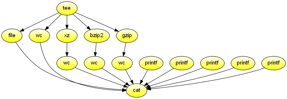
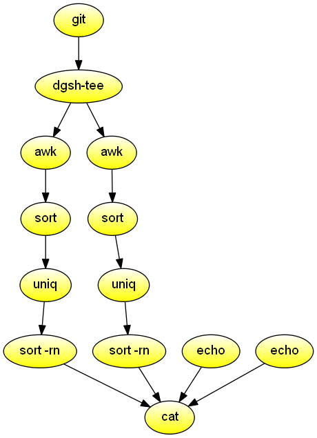
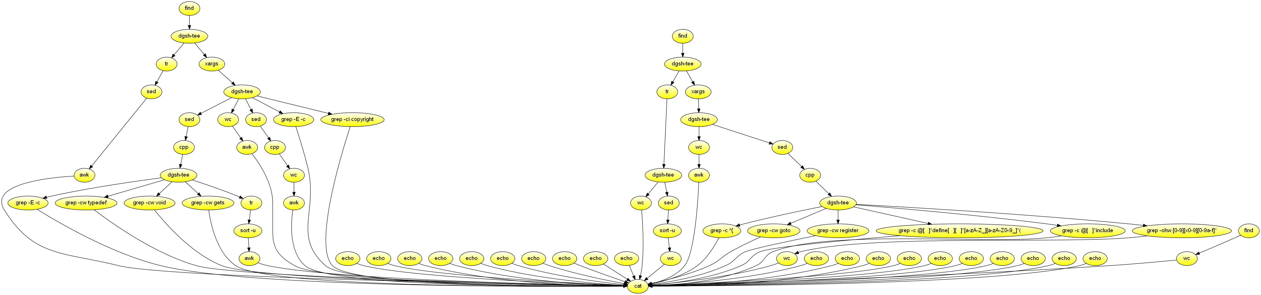
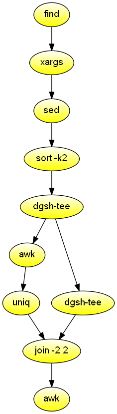
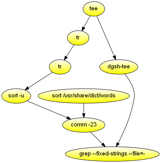
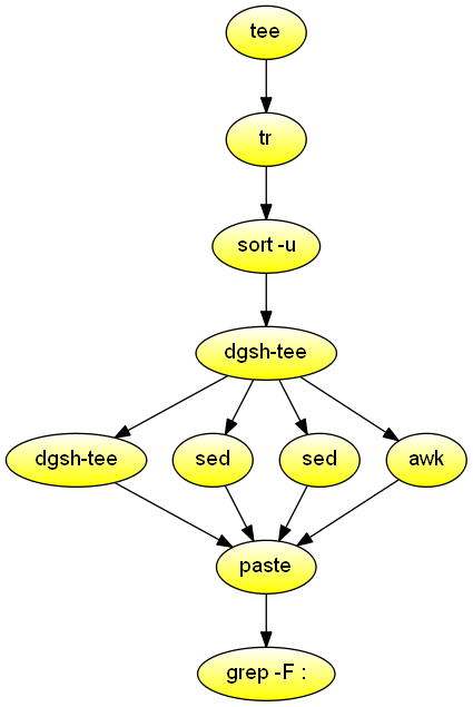
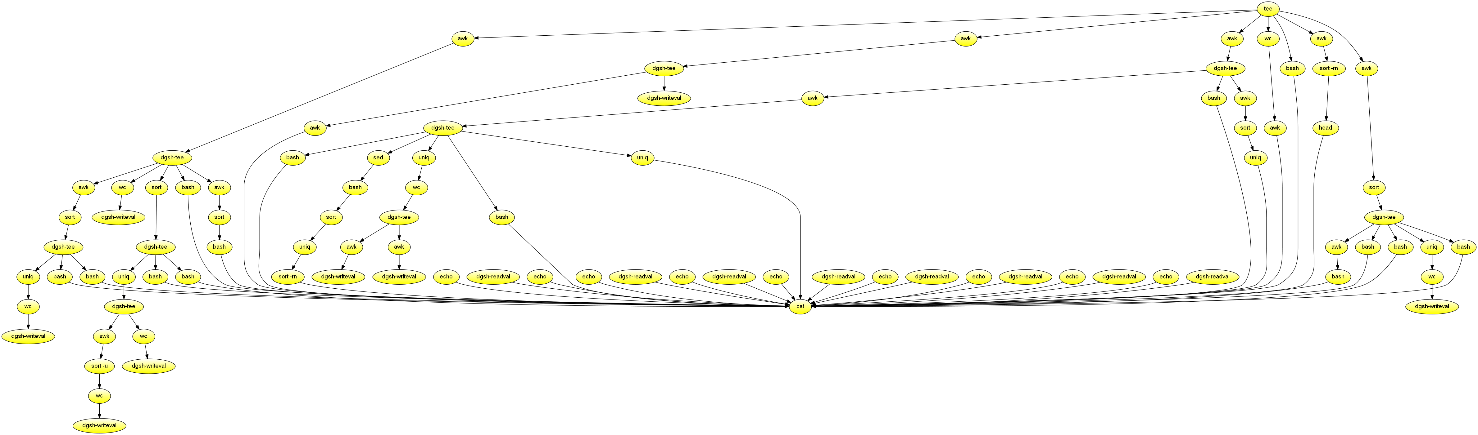
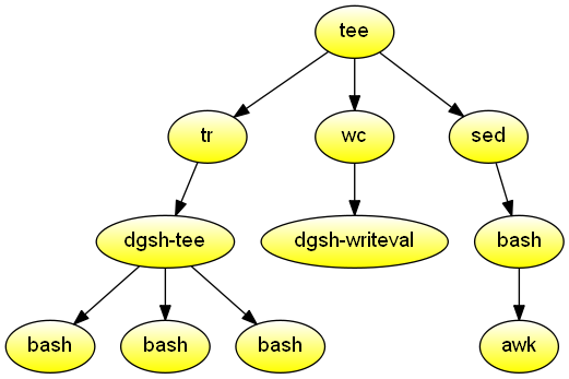
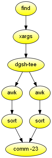
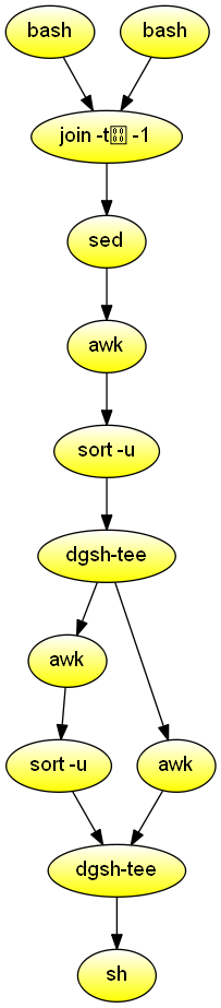
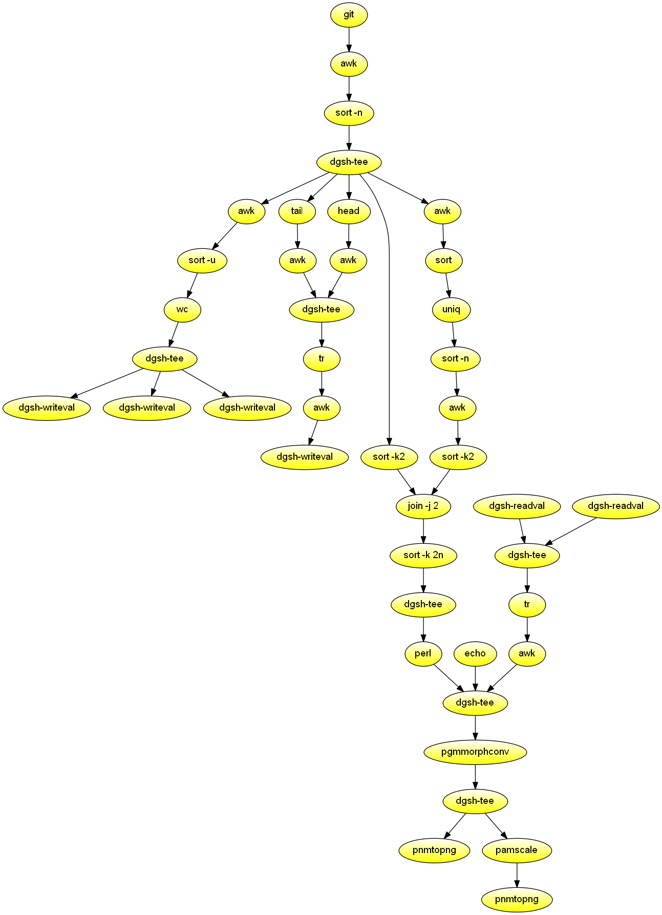
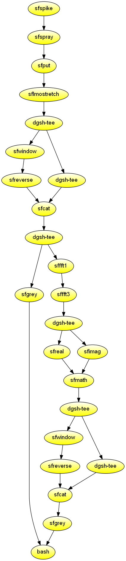
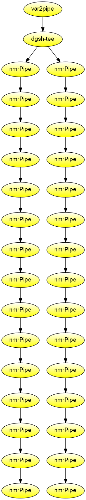
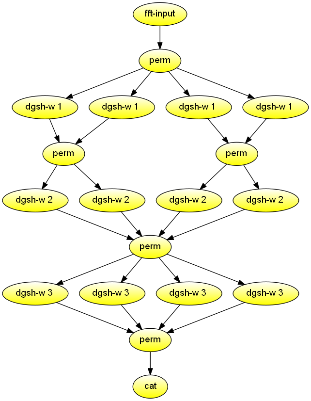

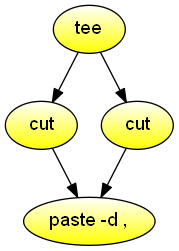
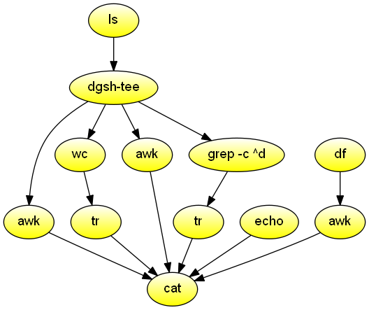


} e^{-\beta E_s}")
 = \sum_s e^{-\beta E_s}")
^k}{Z} \frac{\partial^k}{\partial \beta^k} Z")


 = e^{c \sqrt{\lambda} t} v(x)")
 = e^{i k \cdot x}")


 = \prod_k Z_{\omega_k}(\beta) = \prod_k \frac{1}{1 - e^{- \beta \hbar c \| k \|}}")


 \, d \omega = \frac{V \hbar}{\pi^2 c^3} \frac{\omega^3}{e^{\beta \hbar \omega} - 1} \, d \omega}")


But once you are already on google.com search page, the entire page need not be reloaded. So google would fetch the search results for the new search string via a XHR and update the page.
In fact if you search for https://www.google.com/search?q=wonderland#q=alice, the webpage would first load the search results for 'wonderland' and once the page is loaded, there would be another XHR for 'alice' and the DOM would be updated again with the new results.